Advanced Estimation of ADC and ODF from HARDI Data: A High-Order Approach
550 likes | 710 Vues
This presentation, delivered by Maxime Descoteaux and collaborators, discusses the challenges and advancements in estimating the Apparent Diffusion Coefficient (ADC) and Orientation Distribution Function (ODF) using High Angular Resolution Diffusion Imaging (HARDI). The talk explores limitations of classical Diffusion Tensor Imaging (DTI) when multiple fiber directions coexist in a voxel and proposes high-order formulations to recover fiber crossings through spherical harmonics. Analytical methods and algorithms are outlined for improved accuracy in multi-fiber diffusion characterization.

Advanced Estimation of ADC and ODF from HARDI Data: A High-Order Approach
E N D
Presentation Transcript
ADC and ODF estimation from HARDI Maxime Descoteaux1 Work done with E. Angelino2, S. Fitzgibbons2, R. Deriche1 1. Projet Odyssée, INRIA Sophia-Antipolis, France 2. Physics and Applied Mathematics, Harvard University, USA Max Planck Institute, March 28th 2006
Plan of the talk Introduction Spherical Harmonics Formulation Applications: 1) ADC Estimation 2) ODF Estimation Discussion
Limitation of classical DTI • DTI fails in the presence of many principal directions of different fiber bundles within the same voxel • Non-Gaussian diffusion process True diffusion profile DTI diffusion profile [Poupon, PhD thesis]
High Angular Resolution Diffusion Imaging (HARDI) 162 points 642 points • N gradient directions • We want to recover fiber crossings Solution: Process all discrete noisy samplings on the sphere using high order formulations
High Order Descriptions Seek to characterize multiple fiber diffusion • Apparent Diffusion Coefficient (ADC) • Orientation Distribution Function (ODF) ADC profile Diffusion ODF Fiber distribution
Sketch of the approach Data on the sphere For l = 6, C = [c1, c2 , …, c28] Spherical harmonic description of data ADC ODF ADC ODF
Spherical harmonics Description of discrete data on the sphere Regularization of the coefficients
Spherical harmonicsformulation • Orthonormal basis for complex functions on the sphere • Symmetric when order l is even • We define a real and symmetric modified basis Yj such that the signal [Descoteaux et al. SPIE-MI 06]
Regularization with the Laplace-Beltrami ∆b • Squared error between spherical function F and its smooth version on the sphere ∆bF • SH obey the PDE • We have,
Minimization & -regularization • Minimize (CB - S)T(CB - S) + CTLC => C = (BTB + L)-1BTS • Find best with L-curve method • Intuitively, is a penalty for having higher order terms in the modified SH series => higher order terms only included when needed
Estimation of the ADC Characterize multi-fiber diffusion High order anisotropy measures
Diffusion MRI signal : S(g) Apparent diffusion coefficient ADC profile : D(g) = gTDg
In the HARDI literature… 2 class of high order ADC fitting algorithms: • Spherical harmonic (SH) series [Frank 2002, Alexander et al 2002, Chen et al 2004] • High order diffusion tensor (HODT) [Ozarslan et al 2003, Liu et al 2005]
Summary of algorithm Spherical Harmonic (SH) Series High Order Diffusion Tensor (HODT) HODT D from linear-regression Modified SH basis Yj Least-squares with -regularization M transformation C = (BTB + L)-1BTX D = M-1C [Descoteaux et al. SPIE-MI 06]
Limitations of the ADC • Maxima do not agree with underlying fibers • ADC is in signal space (q-space) HARDI ADC profiles [Campbell et al., McGill University, Canada] Need a function that is in real space with maxima that agree with fibers => ODF
Analytical ODF Estimation Q-Ball Imaging Funk-Hecke Theorem Fiber detection
ODF can be computed directly from the HARDI signal over a single ball Integral over the perpendicular equator = Funk-Radon Transform Q-Ball Imaging (QBI) [Tuch; MRM04] [Tuch; MRM04] ~= ODF
FRT -> ODF Illustration of the Funk-Radon Transform (FRT) Diffusion Signal
Funk-Hecke Theorem [Funk 1916, Hecke 1918]
Funk-Hecke ! Problem: Delta function is discontinuous at 0 ! Recalling Funk-Radon integral
Funk-Hecke formula Delta sequence => Solving the FR integral:Trick using a delta sequence
Final Analytical ODF expression in SH coefficients [Descoteaux et al. ISBI 06]
Biological phantom [Campbell et al. NeuroImage 05] T1-weigthed Diffusion tensors
Corpus callosum - corona radiata - superior longitudinal FA map + diffusion tensors ODFs
Corona radiata diverging fibers - longitudinal fasciculus FA map + diffusion tensors ODFs
Contributions & advantages • SH and HODT description of the ADC • Application to anisotropy measures • Analytical ODF reconstruction • Discrete interpolation/integration is eliminated • Solution for all directions in a single step • Faster than Tuch’s numerical approach by a factor 15 • Spherical harmonic description has powerful properties • Smoothing with Laplace-Beltrami, inner products, integrals on the sphere solved with Funk-Hecke
Perspectives • Tracking and segmentation of fibers using multiple maxima at every voxel • Consider the full diffusion ODF in the tracking and segmentation
Thank you! Key references: • http://www-sop.inria.fr/odyssee/team/ Maxime.Descoteaux/index.en.html -Ozarslan et al. Generalized tensor imaging and analytical relationships between diffusion tensor and HARDI, MRM 50, 2003 -Tuch D. Q-Ball Imaging, MRM 52, 2004
Classical DTI model DTI --> • Brownian motion P of water molecules can be described by a Gaussian diffusion process characterized by rank-2 tensor D (3x3 symmetric positive definite) Diffusion MRI signal : S(q) Diffusion profile : qTDq
Spherical Harmonics (SH) coefficients • In matrix form, S = C*B S : discrete HARDI data 1 x N C : SH coefficients 1 x m = (1/2)(order + 1)(order + 2) B : discrete SH, Yj(m x N (N diffusion gradients and m SH basis elements) • Solve with least-square C = (BTB)-1BTS [Brechbuhel-Gerig et al. 94]
Introduction Limitations of Diffusion Tensor Imaging (DTI) High Angular Resolution Diffusion Imaging (HARDI)
Our Contributions • Spherical harmonics (SH) description of the data • Impose a regularization criterion on the solution • Application to ADC estimation • Direct relation between SH coefficients and independent elements of the high order tensor (HOT) • Application to ODF reconstrution • ODF can be reconstructed ANALITYCALLY • Fast: One step matrix multiplication • Validation on synthetic data, rat biological phantom, knowledge of brain anatomy
High order diffusion tensor (HODT) generalization Rank l = 2 3x3 D = [ Dxx Dyy Dzz Dxy Dxz Dyz ] Rank l = 4 3x3x3x3 D = [ Dxxxx Dyyyy Dzzzz Dxxxy Dxxxz Dyzzz Dyyyz Dzzzx Dzzzy Dxyyy Dxzzz Dzyyy Dxxyy Dxxzz Dyyzz ]
Tensor generalization of ADC • Generalization of the ADC, rank-2 D(g) = gTDg rank-l General tensor Independent elements Dk of the tensor [Ozarslan et al., mrm 2003]
Trick to solve the FR integral • Use a delta sequence n approximation of the delta function in the integral • Many candidates: Gaussian of decreasing variance • Important property
n is a delta sequence 1) 2) =>
Nice trick! 3) =>
Spherical Harmonics • SH • SH PDE • Real • Modified basis
Funk-Hecke Theorem • Key Observation: • Any continuous function f on [-1,1] can be extended to a continous function on the unit sphere g(x,u) = f(xTu), where x, u are unit vectors • Funk-Hecke thm relates the inner product of any spherical harmonic and the projection onto the unit sphere of any function f conitnuous on [-1,1]
z = 1 z = 1000 J0(2z) [Tuch; MRM04] (WLOG, assume u is on the z-axis) Funk-Radon ~= ODF • Funk-Radon Transform • True ODF
55 crossing b = 3000 Field of Synthetic Data b = 1500 SNR 15 order 6 90 crossing
Time Complexity • Input HARDI data |x|,|y|,|z|,N • Tuch ODF reconstruction: O(|x||y||z| N k) (8N) : interpolation point k := (8N) • Analytic ODF reconstruction O(|x||y||z| N R) R := SH elements in basis
Time Complexity Comparison • Tuch ODF reconstruction: • N = 90, k = 48 -> rat data set = 100 , k = 51 -> human brain = 321, k = 90 -> cat data set • Our ODF reconstruction: • Order = 4, 6, 8 -> m = 15, 28, 45 => Speed up factor of ~3
Time complexity experiment • Tuch -> O(XYZNk) • Our analytic QBI -> O(XYZNR) • Factor ~15 speed up
Tuch reconstruction vsAnalytic reconstruction Analytic ODFs Tuch ODFs Difference: 0.0356 +- 0.0145 Percentage difference: 3.60% +- 1.44% [INRIA-McGill]