Channel Estimation from Data
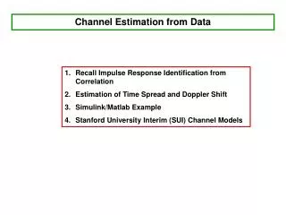
Channel Estimation from Data. Recall Impulse Response Identification from Correlation Estimation of Time Spread and Doppler Shift Simulink/Matlab Example Stanford University Interim (SUI) Channel Models. Estimation of Channel Characteristics from Input - Output data.

Channel Estimation from Data
E N D
Presentation Transcript
Channel Estimation from Data • Recall Impulse Response Identification from Correlation • Estimation of Time Spread and Doppler Shift • Simulink/Matlab Example • Stanford University Interim (SUI) Channel Models
Estimation of Channel Characteristics from Input - Output data. 1. For Linear Time Invariant (LTI) systems: Excite the system with white noise and unit variance and compute thecrosscorrelation between input and output
In matlab: 1. Get data (same length for simplicity): 2. Compute crosscorrelation between input and output: h=xcorr(x,y); If x[n] is white noise, h[n] is the impulse response.
2. For a Linear Time Varying Channel: The impulse response changes with time • Goal: estimate time and frequency spread. • Known: • Sampling frequency • Upper bound on max Doppler Frequency
1. Collect Data and partition in blocks of length : Within each block the channel is almost time invariant X=reshape(x,N,length(x)/N); Y=reshape(x,N,length(y)/N); X,Y =
2. Estimate impulse response in each block : h(:,i)=xcorr(Y(:,i),X(:,i))/N; h = Take the transpose: Each row is an impulse response taken at different times h’ = plot((-N+1:N-1)/Fs, abs(h(:,i)));
3. Compute Power Spectrum on each column of h’ (each row of h) , to determine time variability of the channel (If the channel is Time Invariant all columns of h are the same): time time h’ = time Freq. H=fft(h’); S=H.*conj(H); S =
4. Take the sum over rows for Doppler Spread and sum over columns for Time Spread (fftshift each vector to have “zero” term (sec or Hz) in the middle Sf St Time Resolution: Frequency Resolution: Therefore if we want to a resolution in the doppler spread of (say) 1Hz, we need to collect at least 1 sec of data.
Example: % channel Fs=10^6; % sampling freq. In Hz P=[0,-2,-3]; % attenuations in dB T=[0, 10, 15]*10^(-6); % time delays in sec fd=70; %doppler shift in Hz test_scattering.mdl
Channel Output (Magnitude) with a QPSK Transmitted Signal: t (sec)
sum(S)/NB; sum of each column Time Spread sum(S’)/(2N-1); ave. of each row Frequency Spread