Download
1 / 22
220 likes | 343 Vues
Inferring Mantle Structure in the Past. --- Adjoint method in mantle convection. Lijun Liu Seismo Lab, Caltech Dec. 18, 2006. Present. Plate Tectonics. Seismic Tomography. Dynamic Topography. Geoid. ?. Other Data. Much less is known about the earth’s interior in the past. Past.

E N D
Inferring Mantle Structure in the Past ---Adjoint method in mantle convection Lijun Liu Seismo Lab, Caltech Dec. 18, 2006
Present Plate Tectonics Seismic Tomography Dynamic Topography Geoid ? Other Data Much less is known about the earth’s interior in the past Past
Motivation • Data on earth surface (I) and that of the interior (II) are somehow independent of each other for mantle study. Without exact knowledge of rheology and dynamics, both I and II are not coupled. Plate motion record is not long enough for the “known” subducted slabs to regulate lowermost mantle structures. • Forward modeling has no feedback to the initial state; crude backward integration suffers from accumulated artifacts at thermal boundary layers. • The adjoint method which constrains the initial condition by the output can provide II in the past. • Combination of adjoint method and data I is promising for study of dynamics of solid earth system.
Governing Equations: (continuity) (momentum) (energy) : velocity, P: dynamic pressure, : density, : dynamic viscosity, : thermal diffusivity, H: internal heat source.
Adjoint Equation:integration by part and let (e.g. R. Errico, 1997) The idea of adjoint: (cost function) : error in the initial; Tp: prediction; Td: data Lagrange function: where is the adjoint quantity
Flow Chart Forward run TargetT0 Data T1 1st guess Forward run J Adjoint run
Adjoint method with CitcomS CitcomS is a fully spherical FEM code, solving advection diffusion problems. I developed the adjoint version of CitcomS to realize the time inversion. Surface f = 0.0 f = 0.6 q = 1.27 q = 1.87 CMB
Simple case Boundary Condition: velocity: free slip & non-penetrative temperature:isothermal at top/bot.; zero heat flux on sidewalls. Viscosity:no depth dependence; no temperature dependence Thermal BL:no Reference states: Blank 1st guess
List of the first initial guesses Note: column 2 to 4 describe the anomaly properties. SBI: simple backward integration from present to past
The main feature is always recovered; a better first guess leads to a better recovery. Recovery with SBI first guess has the smallest residual. Higher resolution mesh greatly reduces the residual.
More Complicated Earth Model Viscosity: reference visc. = 1.0e21 (Pa sec) Temperature with thermal boundary layer:
Conclusions about the adjoint method • The adjoint method works well for whole mantle convection models. • The SBI first guess is optimal because it is unique and it leads to a good recovery. However… The adjoint method requires that both model parameters and the present day observation be perfectly known, neither of which is true in general. Present day observation = seismic tomography Model unknowns => mainly rheology (viscosity) !
Theoretically • Numerically h: dynamic topography
Start with a trial viscosity and an estimated temperature from seismic tomography • Adjoint calculation predicted dynamic topography compare with observation • Update temperature and viscosity accordingly
Summary • The dynamic topography, as another constraint, makes the adjoint method practical in real geological problem. • More complicated models are to be tested, e.g. layered viscosity structure, real seismic tomography as observation, etc. • Incorporating plate tectonics history…