Particle Physics
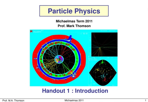
Particle Physics. Michaelmas Term 2011 Prof. Mark Thomson. Handout 1 : Introduction. PART II. PART III. Cambridge Particle Physics Courses. “ Particle and Nuclear Physics ” Prof Ward/Dr Lester. Introductory course. Major Option “ Particle Physics ” Prof Thomson.

Particle Physics
E N D
Presentation Transcript
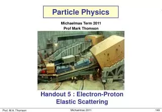
Particle Physics Michaelmas Term 2011 Prof. Mark Thomson Handout 1 : Introduction Michaelmas 2011
PART II PART III Cambridge Particle Physics Courses “Particle and Nuclear Physics” Prof Ward/Dr Lester Introductory course Major Option “Particle Physics” Prof Thomson Covering most Standard Model physics, both experiment and underlying theory Minor Option “Gauge Field Theory” Dr Batley Minor Option “Particle Astrophysics” Profs Efstathiou & Parker The theoretical principles behind the SM The connection between particle physics and cosmology Michaelmas 2011
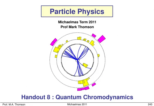
Course Synopsis Handout 1: Introduction, Decay Rates and Cross Sections Handout 2: The Dirac Equation and Spin Handout 3: Interaction by Particle Exchange Handout 4: Electron – Positron Annihilation Handout 5: Electron – Proton Scattering Handout 6: Deep Inelastic Scattering Handout 7: Symmetries and the Quark Model Handout 8: QCD and Colour Handout 9: V-A and the Weak Interaction Handout 10: Leptonic Weak Interactions Handout 11: Neutrinos and Neutrino Oscillations Handout 12: The CKM Matrix and CP Violation Handout 13: Electroweak Unification and the W and Z Bosons Handout 14: Tests of the Standard Model Handout 15: The Higgs Boson and Beyond • Will concentrate on the modern view of particle physics with the emphasis on how theoretical concepts relate to recent experimental measurements • Aim: by the end of the course you should have a good understanding of both aspects of particle physics Michaelmas 2011
Before we start in earnest, a few words on units/notation and a very brief “Part II refresher”… Preliminaries Web-page:www.hep.phy.cam.ac.uk/~thomson/partIIIparticles/ • All course material, old exam questions, corrections, interesting links etc. • Detailed answers will posted after the supervisions (password protected) Format of Lectures/Handouts: • l will derive almost all results from first principles (only a few exceptions). • In places will include some additional theoretical background in non- • examinable appendices at the end of that particular handout. • Please let me know of any typos: thomson@hep.phy.cam.ac.uk Books: • The handouts are fairly complete, however there a number of decent books: • “Particle Physics”, Martin and Shaw (Wiley): fairly basic but good. • “Introductory High Energy Physics”, Perkins (Cambridge): slightly below • level of the course but well written. • “Introduction to Elementary Physics”, Griffiths (Wiley): about right level • but doesn’t cover the more recent material. • “Quarks and Leptons”, Halzen & Martin (Wiley): good graduate level • textbook (slightly above level of this course). Michaelmas 2011
Energy Time Length Momentum Area Mass Energy Time To convert back to S.I. units, need to restore missing factors of and Momentum Length Mass Area Preliminaries: Natural Units • S.I. UNITS: kg m s are a natural choice for “everyday” objects e.g. M(Prescott) ~ 250 kg • not very natural in particle physics • instead use Natural Units based on the language of particle physics • From Quantum Mechanics - the unit of action : • From relativity - the speed of light: c • From Particle Physics - unit of energy: GeV (1 GeV ~ proton rest mass energy) • Units become (i.e. with the correct dimensions): • Simplify algebra by setting: • Now all quantities expressed in powers of GeV Michaelmas 2011
and Unless otherwise stated, Natural Units are used throughout these handouts, , , etc. Preliminaries: Heaviside-Lorentz Units • Electron chargedefined by Force equation: • In Heaviside-Lorentz units set NOW: electric charge has dimensions • Since Michaelmas 2011
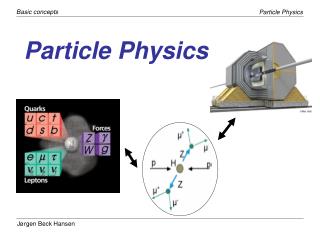
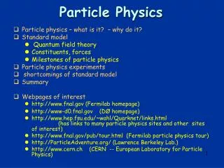
Review of The Standard Model Particle Physics is the study of: • MATTER: the fundamental constituents of the universe - the elementary particles • FORCE: the fundamental forces of nature, i.e. the interactions between the elementary particles Try to categorise the PARTICLES and FORCES in as simple and fundamental manner possible • Current understanding embodied in the STANDARD MODEL: • Forces between particles due to exchange of particles • Consistent with all current experimental data ! • But it is just a “model” with many unpredicted parameters, • e.g. particle masses. • As such it is not the ultimate theory (if such a thing exists), there • are many mysteries. Michaelmas 2011
Matter in the Standard Model • In the Standard Model the fundamental “matter” is described by point-like spin-1/2 fermions The masses quoted for the quarks are the “constituent masses”, i.e. the effective masses for quarks confined in a bound state • In the SM there are three generations – the particles in each generation • are copies of each other differing only in mass. (not understood why three). • The neutrinos are much lighter than all other particles (e.g. n1 has m<3 eV) • – we now know that neutrinos have non-zero mass (don’t understand why • so small) Michaelmas 2011
Forces in the Standard Model • Forces mediated by the exchange of spin-1Gauge Bosons g g • Fundamental interaction strength is given by charge g. • Related to the dimensionlesscoupling “constant” e.g. QED (both gand aare dimensionless, but gcontains a “hidden” ) • In Natural Units • Convenient to express couplings in terms of a which, being genuinely dimensionless does not depend on the system of units (this is not true for the numerical value for e) Michaelmas 2011
Interaction of gauge bosons with fermions described by SM vertices • Properties of the gauge bosons and nature of the interaction between the bosons and fermions determine the properties of the interaction STRONG EM WEAK CC WEAK NC q q m+ m+ d q u g q g W Z Only quarks All charged fermions All fermions All fermions Never changes flavour Always changes flavour Never changes flavour Never changes flavour Standard Model Vertices Michaelmas 2011
e– e– m+ e+ g g m– e– q q • IMPORTANT POINTS TO REMEMBER: INITIAL FINAL • “time” runs from left – right, only in sense that: • LHS of diagram is initial state • RHS of diagram is final state • Middle is “how it happened” • anti-particle arrows in –ve “time” direction • Energy, momentum, angular momentum, etc. • conserved at all interaction vertices • All intermediate particles are “virtual” • i.e. (handout 3) m+ e+ g m– e– “time” Feynman Diagrams • Particle interactions described in terms of Feynman diagrams e.g. scattering e.g. annihilation Michaelmas 2011
Invariant mass Phase or Four vectors written as either: or Three vectors written as: Special Relativity and 4-Vector Notation • Will use 4-vector notation withas the time-like component, e.g. (contravariant) (covariant) with • In particle physics, usually deal with relativistic particles. Requireall • calculations to be Lorentz Invariant. L.I. quantities formed from 4-vector • scalar products, e.g. • A few words on NOTATION Four vector scalar product: or Quantities evaluated in the centre of mass frame: etc. Michaelmas 2011
3 1 2 e– e– m+ 4 e+ g g m– e– e– e– Mandelstam s, t and u • In particle scattering/annihilation there are three particularly useful Lorentz Invariant quantities: s, t and u • Consider the scattering process • (Simple) Feynman diagrams can be categorised according to the four-momentum of the exchanged particle e– e– g e– e– s-channel t-channel u-channel • Can define three kinematic variables: s, t and u from the following four vector • scalar products (squared four-momentum of exchanged particle) Michaelmas 2011
m+ e+ g m– e– Example: Mandelstam s, t and u Note: (Question 1) • e.g. Centre-of-mass energy, s: • This is a scalar product of two four-vectors Lorentz Invariant • Since this is a L.I. quantity, can evaluate in any frame. Choose the • most convenient, i.e. the centre-of-mass frame: • Hence is the total energy of collision in the centre-of-mass frame Michaelmas 2011
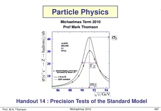
Many beautiful experimental measurements • precise theoretical predictions challenged by precise measurements From Feynman diagrams to Physics Particle Physics = Precision Physics • Particle physics is about building fundamental theories and testing their predictions against precise experimental data • Dealing with fundamental particles and can make very precise theoretical • predictions– not complicated by dealing with many-body systems • For all its flaws, the Standard Model describes all experimental data ! • This is a (the?)remarkable achievement of late 20th century physics. Requires understanding of theory and experimental data • Part II : Feynman diagrams mainly used to describe how particles interact • will use Feynman diagrams and associated Feynman rules to perform calculations for many processes • hopefully gain a fairly deep understanding of the Standard Model and how it explains all current data • Part III: • Before we can start, need calculations for: • Interaction cross sections; • Particle decay rates; Michaelmas 2011
Calculate transition rates from Fermi’s Golden Rule is number of transitions per unit time from initial state to final state –not Lorentz Invariant ! is Transition Matrix Element is the perturbing Hamiltonian is density of final states Cross Sections and Decay Rates • In particle physics we are mainly concerned • with particle interactions and decays, i.e. • transitions between states • these are the experimental observables of particle physics • Rates depend on MATRIX ELEMENT and DENSITY OF STATES the ME contains the fundamental particle physics just kinematics Michaelmas 2011
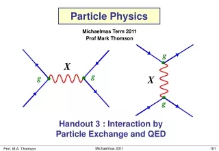
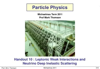
m+ e+ g e– e– m– e– q q • Need relativistic calculation of interaction Matrix Element: Interaction by particle exchange and Feynman rules • Need relativistic treatment of spin-half particles: Dirac Equation The first five lectures • Aiming towards a proper calculation of decay and scattering processes Will concentrate on: • e+e– m+m– • e– q e– q (e– qe– q to probe proton structure) • Need relativistic calculations of particle decay rates and cross sections: + and a few mathematical tricks along, e.g. the Dirac Delta Function Michaelmas 2011
1 i q 2 as Particle Decay Rates • Consider the two-body decay • Want to calculate the decay rate in first order • perturbation theory using plane-wave descriptions • of the particles (Born approximation): where N is the normalisation and For decay rate calculation need to know: • Wave-function normalisation • Transition matrix element from perturbation theory • Expression for the density of states All in a Lorentz Invariant form • First consider wave-function normalisation • Previously (e.g. part II) have used a non-relativistic formulation • Non-relativistic: normalised to one particle in a cube of side Michaelmas 2011
a a a Non-relativistic Phase Space (revision) • Apply boundary conditions ( ): • Wave-function vanishing at box boundaries • quantised particle momenta: • Volume of single state in momentum space: • Normalising to one particle/unit volume gives • number of states in element: • Therefore density of states in Golden rule: with • Integrating over an elemental shell in • momentum-space gives Michaelmas 2011
a Dirac d Function • In the relativistic formulation of decay rates and cross sections we will make • use of the Dirac d function: “infinitely narrow spike of unit area” • Any function with the above properties can represent e.g. (an infinitesimally narrow Gaussian) • In relativistic quantum mechanics delta functions prove extremely useful • for integrals over phase space, e.g. in the decay and express energy and momentum conservation Michaelmas 2011
x • Now express in terms of where x • We will soon need an expression for the delta functionof a function • Start from the definition of a delta function and then change variables • From properties of the delta function (i.e. here only • non-zero at ) • Rearranging and expressing the RHS as a delta function (1) Michaelmas 2011
1 i q since 2 The Golden Rule revisited • Rewrite the expression for density of states using a delta-function Note : integrating over all final state energies but energy conservation now taken into account explicitly by delta function • Hence the golden rule becomes: the integral is over all“allowed” final states of any energy • For dnin a two-body decay, only need to consider one particle : mom. conservation fixes the other • However, can include momentum conservation explicitly by integrating over the momenta of both particles and using another d-fn Mom. cons. Energy cons. Density of states Michaelmas 2011
When considering relativistic effects, volume contractsby a a a a a/g a Lorentz Invariant Phase Space • In non-relativistic QM normalise to one particle/unit volume: • Particle density therefore increases by • Conclude that a relativistic invariant wave-function normalisation needs to be proportional to E particles per unit volume • Usual convention: Normalise to 2E particles/unit volume • Previously used normalised to 1 particle per unit volume • Hence is normalised to per unit volume • DefineLorentz Invariant Matrix Element, , in terms of the wave-functions • normalised to particles per unit volume Michaelmas 2011
Now expressing in terms of gives This form of is simply a rearrangement of the original equation but the integral is now frame independent (i.e. L.I.) • For the two body decay Note: uses relativistically normalised wave-functions. It is Lorentz Invariant is the Lorentz Invariant Phase Space for each final state particle the factor of arises from the wave-function normalisation (prove this in Question 2) is inversely proportional to Ei, the energy of the decaying particle. This is exactly what one would expect from time dilation (Ei = gm). Energy and momentum conservation in the delta functions Michaelmas 2011
1 i q 2 • Integrating over using the d-function: For convenience, here is written as Decay Rate Calculations • Because the integral is Lorentz invariant (i.e. frame independent) it can be evaluated in any frame we choose. The C.o.M. frame is most convenient • In the C.o.M. frame and now since the d-function imposes • Writing Michaelmas 2011
1 i q • imposes energy conservation. 2 • Which can be written • in the form (2) where and Note: • determines the C.o.M momenta of • the two decay products i.e. for • Eq. (2) can be integrated using the property of d – function derived earlier (eq. (1)) where is the value for which • All that remains is to evaluate Michaelmas 2011
In the particle’s rest frame • can be obtained from giving: • But from , i.e. energy conservation: (3) VALID FOR ALL TWO-BODY DECAYS ! (Question 3) (now try Questions 4 & 5) Michaelmas 2011
no of interactions per unit time per target s = incident flux s ds ds no of particles per sec/per target into dW = d... dW incident flux q Cross section definition Flux = number of incident particles/ unit area/unit time • The “cross section”, s, can be thought of as theeffectivecross- • sectional area of the target particles for the interaction to occur. • In general this has nothing to do with the physical size of the • target although there are exceptions, e.g. neutron absorption here is the projective area of nucleus Differential Cross section or generally e– e– with p integrate over all other particles Michaelmas 2011
In time dta particle of type a traverses region containing va vb A particles of type b s A nb v s Rate per particle of type a = example • Consider a single particle of type a with velocity,va, traversing a region of area • A containing nb particles of type b per unit volume • Interaction probability obtained from effective cross-sectional area occupied by the particles of type b • Interaction Probability = • Consider volumeV, total reaction rate = = • As anticipated: Rate = Flux x Number of targets x cross section Michaelmas 2011
the parts are not Lorentz Invariant Cross Section Calculations 3 • Consider scattering process 1 2 • Start from Fermi’s Golden Rule: 4 where is the transition matrix for a normalisation of 1/unit volume • Now • For 1 target particle per unit volume Michaelmas 2011
To obtain a Lorentz Invariant form use wave-functions normalised to particles • per unit volume • Again define L.I. Matrix element • The integral is now written in a Lorentz invariant form • The quantity can be written in terms of a four-vector scalar product and is therefore also Lorentz Invariant (the Lorentz Inv. Flux) (see appendix I) • Consequently cross section is a Lorentz Invariant quantity Two special cases of Lorentz Invariant Flux: • Centre-of-Mass Frame • Target (particle 2) at rest Michaelmas 2011
3 1 2 4 • The integral is exactly the same integral that appeared in the particle decay calculation but with replaced by 22 Body Scattering in C.o.M. Frame • We will now apply above Lorentz Invariant formula for the • interaction cross section to the most common cases used • in the course. First consider 22 scattering in C.o.M. frame • Start from • Here Michaelmas 2011
1 e– e– 3 • In the case of elastic scattering 2 m+ m+ 4 • For calculating the total cross-section (which is Lorentz Invariant) the result on • the previous page (eq. (4)) is sufficient. However, it is not so useful for calculating • the differential cross section in a rest frame other than the C.o.M: because the angles in refer to the C.o.M frame • For the last calculation in this section, we need to find a L.I. expression for • Start by expressing in terms of Mandelstam t i.e. the square of the four-momentum transfer e– e– Product of four-vectors therefore L.I. Michaelmas 2011
Want to express in terms of Lorentz Invariant x 3 1 z 2 4 giving • Finally, integrating over (assuming no dependence of ) gives: where • In C.o.M. frame: therefore hence Michaelmas 2011
Lorentz Invariant differential cross section • All quantities in the expression for are Lorentz Invariant and therefore, it applies to any rest frame. It should be noted that is a constant, fixed by energy/momentum conservation • As an example of how to use the invariant expression we will consider elastic scattering in the laboratory frame in the limit where we can neglect the mass of the incoming particle E1 m2 e.g. electron or neutrino scattering In this limit Michaelmas 2011
3 3 1 2 q 1 4 4 2 Integrating over e– e– X X so here 22 Body Scattering in Lab. Frame • The other commonly occurring case is scattering from a fixed target in the • Laboratory Frame (e.g. electron-proton scattering) • First take the case of elastic scattering at high energy where the mass • of the incoming particles can be neglected: e.g. • Wish to express the cross section in terms of scattering angle of the e– therefore • The rest is some rather tedious algebra…. start from four-momenta But from (E,p) conservation and, therefore, can also express t in terms of particles 2 and 4 Michaelmas 2011
Particle 1 massless In limit Note E1 is a constant (the energy of the incoming particle) so • Equating the two expressions for tgives so using gives Michaelmas 2011
In this equation, E3 is a function of q : giving General form for 22 Body Scattering in Lab. Frame • The calculation of the differential cross section for the case where m1 can not be neglected is longer and contains no more “physics”(see appendix II). It gives: Again there is only one independent variable, q, which can be seen from conservation of energy i.e. is a function of Michaelmas 2011
Summary • Used a Lorentz invariant formulation of Fermi’s Golden Rule to derive decay rates and cross-sections in terms of the Lorentz Invariant Matrix Element(wave-functions normalised to 2E/Volume) Main Results: • Particle decay: Where is a function of particle masses • Scattering cross section in C.o.M. frame: • Invariant differential cross section (valid in all frames): Michaelmas 2011
Summary cont. • Differential cross section in the lab. frame (m1=0) • Differential cross section in the lab. frame (m1≠0) with Summary of the summary: • Have now dealt with kinematics of particle decays and cross sections • The fundamental particle physics is in the matrix element • The above equations are the basis for all calculations that follow Michaelmas 2011
Appendix I : Lorentz Invariant Flux NON-EXAMINABLE a b • Collinear collision: To show this is Lorentz invariant, first consider Giving Michaelmas 2011
3 2 q 1 4 Appendix II : general 22 Body Scattering in lab frame NON-EXAMINABLE again But now the invariant quantity t: Michaelmas 2011
Which gives To determine dE3/d(cosq), first differentiate (AII.1) Then equate to give Differentiate wrt. cosq Using (1) (AII.2) Michaelmas 2011
It is easy to show and using (AII.2) obtain Michaelmas 2011