Download
1 / 21
240 likes | 920 Vues
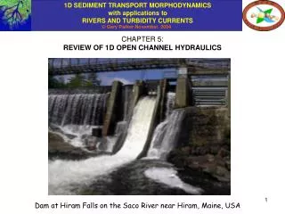
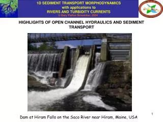
HIGHLIGHTS OF OPEN CHANNEL HYDRAULICS AND SEDIMENT TRANSPORT. Dam at Hiram Falls on the Saco River near Hiram, Maine, USA. SIMPLIFICATION OF CHANNEL CROSS-SECTIONAL SHAPE.

E N D
HIGHLIGHTS OF OPEN CHANNEL HYDRAULICS AND SEDIMENT TRANSPORT Dam at Hiram Falls on the Saco River near Hiram, Maine, USA
SIMPLIFICATION OF CHANNEL CROSS-SECTIONAL SHAPE River channel cross sections have complicated shapes. In a 1D analysis, it is appropriate to approximate the shape as a rectangle, so that B denotes channel width and H denotes channel depth (reflecting the cross-sectionally averaged depth of the actual cross-section). As was seen in Chapter 3, natural channels are generally wide in the sense that Hbf/Bbf << 1, where the subscript “bf” denotes “bankfull”. As a result the hydraulic radius Rh is usually approximated accurately by the average depth. In terms of a rectangular channel,
THE SHIELDS NUMBER: A KEY DIMENSIONLESS PARAMETER QUANTIFYING SEDIMENT MOBILITY b = boundary shear stress at the bed (= bed drag force acting on the flow per unit bed area) [M/L/T2] c = Coulomb coefficient of resistance of a granule on a granular bed [1] Recalling that R = (s/) – 1, the Shields Number * is defined as It can be interpreted as a ratio scaling the ratio impelling force of flow drag acting on a particle to the Coulomb force resisting motion acting on the same particle, so that The characterization of bed mobility thus requires a quantification of boundary shear stress at the bed.
QUANTIFICATION OF BOUNDARY SHEAR STRESS AT THE BED U = cross-sectionally averaged flow velocity ( depth-averaged flow velocity in the wide channels studied here) [L/T] u* = shear velocity [L/T] Cf = dimensionless bed resistance coefficient [1] Cz = dimensionless Chezy resistance coefficient [1]
RESISTANCE RELATIONS FOR HYDRAULICALLY ROUGH FLOW Keulegan (1938) formulation: where = 0.4 denotes the dimensionless Karman constant and ks = a roughness height characterizing the bumpiness of the bed [L]. Manning-Strickler formulation: where r is a dimensionless constant between 8 and 9. Parker (1991) suggested a value of r of 8.1 for gravel-bed streams. Roughness height over a flat bed (no bedforms): where Ds90 denotes the surface sediment size such that 90 percent of the surface material is finer, and nk is a dimensionless number between 1.5 and 3. For example, Kamphuis (1974) evaluated nk as equal to 2.
COMPARISION OF KEULEGAN AND MANNING-STRICKLER RELATIONS r = 8.1 Note that Cz does not vary strongly with depth. It is often approximated as a constant in broad-brush calculations.
TEST OF RESISTANCE RELATION AGAINST MOBILE-BED DATA WITHOUT BEDFORMS FROM LABORATORY FLUMES
NORMAL FLOW Normal flow is an equilibrium state defined by a perfect balance between the downstream gravitational impelling force and resistive bed force. The resulting flow is constant in time and in the downstream, or x direction. • Parameters: • x = downstream coordinate [L] • H = flow depth [L] • U = flow velocity [L/T] • qw = water discharge per unit width [L2T-1] • B = width [L] • Qw = qwB = water discharge [L3/T] • g = acceleration of gravity [L/T2] • = bed angle [1] tb = bed boundary shear stress [M/L/T2] • S = tan = streamwise bed slope [1] • (cos 1; sin tan S) • = water density [M/L3] As can be seen from Chapter 3, the bed slope angle of the great majority of alluvial rivers is sufficiently small to allow the approximations
NORMAL FLOW contd. Conservation of water mass (= conservation of water volume as water can be treated as incompressible): Conservation of downstream momentum: Impelling force (downstream component of weight of water) = resistive force Reduce to obtain depth-slope product rule for normal flow:
ESTIMATED CHEZY RESISTANCE COEFFICIENTS FOR BANKFULL FLOW BASED ON NORMAL FLOW ASSUMPTION FOR u* The plot below is from Chapter 3
RELATION BETWEEN qw, S and H AT NORMAL EQUILIBRIUM Reduce the relation for momentum conservation b = gHS with the resistance form b = CfU2: Generalized Chezy velocity relation or Further eliminating U with the relation for water mass conservation qw = UH and solving for flow depth: Relation for Shields stress at normal equilibrium: (for sediment mobility calculations)
ESTIMATED SHIELDS NUMBERS FOR BANKFULL FLOW BASED ON NORMAL FLOW ASSUMPTION FOR b The plot below is from Chapter 3
RELATIONS AT NORMAL EQUILIBRIUM WITH MANNING-STRICKLER RESISTANCE FORMULATION Solve for H to find Solve for U to find Manning-Strickler velocity relation (n = Manning’s “n”) Relation for Shields stress at normal equilibrium: (for sediment mobility calculations)
BUT NOT ALL OPEN-CHANNEL FLOWS ARE AT OR CLOSE TO EQUILIBRIUM! And therefore the calculation of bed shear stress as b = gHS is not always accurate. In such cases it is necessary to compute the disquilibrium (e.g. gradually varied) flow and calculate the bed shear stress from the relation Flow over a free overfall (waterfall) usually takes the form of an M2 curve. Flow into standing water (lake or reservoir) usually takes the form of an M1 curve. A key dimensionless parameter describing the way in which open-channel flow can deviate from normal equilibrium is the Froude number Fr:
NON-STEADY, NON-UNIFORM 1D OPEN CHANNEL FLOWS: St. Venant Shallow Water Equations • x = boundary (bed) attached nearly horizontal coordinate [L] • y = upward normal coordinate [L] • = bed elevation [L] S = tan - /x [1] H = normal (nearly vertical) flow depth [L] Here “normal” means “perpendicular to the bed” and has nothing to do with normal flow in the sense of equilibrium. Bed and water surface slopes exaggerated below for clarity. Relation for water mass conservation (continuity): Relation for momentum conservation:
flow subcritical supercritical HYDRAULIC JUMP Supercritical (Fr >1) to subcritical (Fr < 1) flow.
ILLUSTRATION OF BEDLOAD TRANSPORT Double-click on the image to see a video clip of bedload transport of 7 mm gravel in a flume (model river) at St. Anthony Falls Laboratory, University of Minnesota. (Wait a bit for the channel to fill with water.) Video clip from the experiments of Miguel Wong. rte-bookbedload.mpg: to run without relinking, download to same folder as PowerPoint presentations.
ILLUSTRATION OF MIXED TRANSPORT OF SUSPENDED LOAD AND BEDLOAD Double-click on the image to see the transport of sand and pea gravel by a turbidity current (sediment underflow driven by suspended sediment) in a tank at St. Anthony Falls Laboratory. Suspended load is dominant, but bedload transport can also be seen. Video clip from experiments of Alessandro Cantelli and Bin Yu. rte-bookturbcurr.mpg: to run without relinking, download to same folder as PowerPoint presentations.
PARAMETERS CHARACTERIZING SEDIMENT TRANSPORT qb = Volume bedload transport rate per unit width [L2/T] qs = Volume suspended load transport rate per unit width [L2/T] qt = qb + qs = volume total bed material transport rate per unit width [L2/T] qw = Volume wash load transport rate per unit width [L2/T] = water density [M/L3] s = sediment density [M/L3] R = (s/) – 1 = sediment submerged specific gravity [1] D = characteristic sediment size (e.g. Ds50) [L] * = dimensionless Shields number, = (HS)/(RD) for normal flow [1] Dimensionless Einstein number for bedload transport Dimensionless Einstein number for total bed material transport
SOME GENERIC RELATIONS FOR SEDIMENT TRANSPORT BEDLOAD TRANSPORT RELATIONS (e.g. gravel-bed stream) Wong’s modified version of the relation of Meyer-Peter and Müller (1948) Parker’s (1979) approximation of the Einstein (1950) relation TOTAL BED MATERIAL LOAD TRANSPORT RELATION (e.g. sand-bed stream) Engelund-Hansen relation (1967)
REFERENCES Chaudhry, M. H., 1993, Open-Channel Flow, Prentice-Hall, Englewood Cliffs, 483 p. Crowe, C. T., Elger, D. F. and Robertson, J. A., 2001, Engineering Fluid Mechanics, John Wiley and sons, New York, 7th Edition, 714 p. Gilbert, G.K., 1914, Transportation of Debris by Running Water, Professional Paper 86, U.S. Geological Survey. Jain, S. C., 2000, Open-Channel Flow, John Wiley and Sons, New York, 344 p. Kamphuis, J. W., 1974, Determination of sand roughness for fixed beds, Journal of Hydraulic Research, 12(2): 193-202. Keulegan, G. H., 1938, Laws of turbulent flow in open channels, National Bureau of Standards Research Paper RP 1151, USA. Henderson, F. M., 1966, Open Channel Flow, Macmillan, New York, 522 p. Meyer-Peter, E., Favre, H. and Einstein, H.A., 1934, Neuere Versuchsresultate über den Geschiebetrieb, Schweizerische Bauzeitung, E.T.H., 103(13), Zurich, Switzerland. Meyer-Peter, E. and Müller, R., 1948, Formulas for Bed-Load Transport, Proceedings, 2nd Congress, International Association of Hydraulic Research, Stockholm: 39-64. Parker, G., 1991, Selective sorting and abrasion of river gravel. II: Applications, Journal of Hydraulic Engineering, 117(2): 150-171. Vanoni, V.A., 1975, Sedimentation Engineering, ASCE Manuals and Reports on Engineering Practice No. 54, American Society of Civil Engineers (ASCE), New York. Wong, M., 2003, Does the bedload equation of Meyer-Peter and Müller fit its own data?, Proceedings, 30th Congress, International Association of Hydraulic Research, Thessaloniki, J.F.K. Competition Volume: 73-80.