Exploring Built-in Functions in MATLAB for Engineering Applications
220 likes | 366 Vues
This chapter introduces the rich array of predefined built-in functions available in MATLAB, essential for engineering computations. Key functions such as sqrt, sin, cos, and others are explained, along with their operations on scalars, vectors, and matrices. The "help" command is highlighted for accessing documentation. Moreover, specialized toolboxes for various fields are discussed, alongside guidance for writing custom functions. The section also covers valuable mathematical functions, random number generators, and matrix manipulations, providing a comprehensive understanding for effective MATLAB usage.

Exploring Built-in Functions in MATLAB for Engineering Applications
E N D
Presentation Transcript
Chapter 3 Review: Built In MATLAB Functions Introduction to MATLAB 7 Engineering 161
Predefined MATLAB functions • MATLAB is rich in predefined or built in functions that you can use in your expressions and calculations; x = [16, 25, 9, 4]; y = sqrt ( x ); yields the vector y with values [4, 5, 3, 2] sqrt is a built in MATLAB function that operates on scalars and vectors and matrices.
Predefined MATLAB functions II • Use the “help” command to learn how to use a particular function >> help sqrt • Use “MATLAB Help” feature to see a list of all MATLAB functions that are available and read the documentation about each of them. • MATLAB functions are varied and powerful and can be nested, sqrt(sin(abs(x))) where x can be a matrix, vector or scalar.
Using MATLAB functions • MATLAB functions come “built in” to MATLAB, sqrt, sin, abs, max, exp, etc. • MATLAB functions come in specialized “toolboxes” for special fields of work; the financial toolbox, statistical toolbox, symbolic math toolbox are examples. • And, you will be able to write your own functions and use them just like built in ones.
abs(x) absolute value sqrt(x) square root round(x) rounds to nearest fix(x) truncates toward 0 floor(x) rounds down ceil(x) rounds up sign(x) sign of x rem(x,y) remainder of x/y exp(x)e raised to x power log(x) natural log of x log10(x) log to the base 10 log2(x) log to the base 2 Some Elementary Math and Rounding Functions
Some Trigonometric Functions • sin(x) computes the sine of x, x in radians, • cos(x) computes the cosine of x, x in radians • tan(x) computes the tangent of x, x in radians • asin(y) computes the inverse sine, -1 < x < +1 • atan(y) computes the inverse tangent, i.e., computes the angle whose tangent is y • Notice that MATLAB wants angles to be expressed in radians, not degrees. To convert use the relationship 1 degree = pi/180 radians angle_radians = angle_degrees*(pi/180) angle_degrees = angle_radians*(180/pi) (sind(x) permits x to be in degrees)
Other Useful Elementary Analysis Functions • See our text for more detailed explanations; see Appendix A for a list of some of the MATLAB functions. • max(x), min(x), mean(x), median(x), std(x), sum(x), prod(x), cumsum(x), cumprod(x), sort(x), size(x), length(x) are just a few. • Note that x may be a vector (row or column) or a matrix. For matrices, functions typically work on the columns of the matrix to yield their results. (Always best to use help feature to check and make sure.)
Functions with Multiple Outputs • Some functions return multiple results, for example, consider the max function; • [a,b] = max(x) where x is a row vector of arbitrary length, returns two values, a will be the maximum value while b will be the index in the row vector of the maximum value
Functions with Multiple Outputs % x = [2,4,6.5,-3, 7.9, 4.1]; [a,b] = max(x) a = 7.9 b = 5
Functions used in Discrete Mathematics • factor(x)- finds the factors of x • gcd(x,y)- finds the greatest common denominator of x and y • lcm(x,y)- finds the least common multiple of x and y • rats(x)- represents x as a fraction • factorial(x)- for x=4 implies factorial(x) = 24 • primes(x)- finds all the prime numbers < x • isprime(x)- checks to see if x is a prime number, function returns 1 if yes; 0 if no.
Random Number Generators I • MATLAB contains two random number generators, rand(n,m) for uniformly distributed random numbers and randn(n,m) for normal or Gaussian distributed random numbers. • Random number sequences can be scaled for different mean and standard deviation requirements. • Sequences of random numbers are often used in engineering problem solving. • x = 10*rand(1,100) – 5; creates a row vector x with 100 random numbers uniformly distributed between -5 and 5. • Enter the above command followed by the command plot (x) to see what happens.
Random Number Generators II • rand(n)- nxn matrix uniformly distributed (0 to 1) • rand(m,n)- mxn matrix uniformly distributed (0 to 1) • randn(n)- nxn matrix Gaussian distributed • randn(mxn)- mxn matrix Gaussian distributed • mean (x)- computes mean value of a vector x • median(x)- finds the median of the elements of x • std(x)- computes the standard deviation of the elements of x • var(x)- computes the variance of the elements of x
More on Matrices • We’ve seen ways to define matrices; A = [1,3,5] A = [1 3 5] are equivalent t = -1:0.5:2 yields t = [-1, -0.5, 0, .5, 1, 1.5, 2] B = [1,2,5;3,4,6] yields the 2X3 matrix of two rows and three columns x = linspace(-5,5,10) creates the vector x of 10 values equally spaced between -5 and 5
More on Matrices II • Also consider >> a = [3,5] >> b = [1,a] creates the row vector where b = [1,3,5] >> b(2) is the scalar with value 3 >> a' is the column vector, 2 rows and one column (we say “a transpose”)
More on the colon operator • For M=[1,2,3,4,5;2,3,4,5,6;3,4,5,6,7] • x = M(:,1) is the column vector, the 1st column of M • x = M(:,3) is a column vector, the 3rd column of M • y = M(2,:) is a row vector, the second row of M • w = M(2:3,:) is a 2 rows and 5 columns matrix made up of the last two rows of M • w = M(2:3,4:5) is a 2 rows and 2 columns matrix made up the elements, [5,6;6,7] • And don’t forget, z = M(2,4), then z = 5
Special Values • MATLAB includes a number of predefined constants, special values and special matrices. • Some examples include, pi, i and j {sqrt (-1)}, Inf, NaN, clock, date, eps, and ans. • MATLAB allows the following statement, pi = 3, but be careful, pi will take in the value of 3 not 3.14159.. until it is reset to the value of pi. Clearing the Workspace reestablishes the value of pi. • Same is true for built in function names, avoid it.
Other Useful Functions • abs(z)- computes the absolute value of a complex number • angle(z)- computes the angle in radians of a complex number used in its polar representation • complex(x,y)- generates a complex number, you can also write z = 5 + i*7 • real(z)- extracts the real part of a complex number • imag(z)- extracts the imaginary component of a complex number • isreal(z)- determines if z is real or not • conj(z)- generates the complex conjugate of z
Other Functions • See the Table on pages 112 - 113 for a list of basic functions described in Chp. 3. This is a very small subset of MATLAB built in functions. Don’t forget to use the Help feature to learn more about these functions and to find functions that will help you solve problems. • Also see Table 3.16 on page 110 for special MATLAB functions and symbols.
Example; Problem 3.3 % Joe Mixsell % Problem 3.3 % Calculate the number of rabbits after 10 years with a % starting number of 100 and breeding at a rate of 90 percent/yr R = 0.9; % Breeding rate P0 = 100; % Initial population t = 0:1:10; % 10 years in increments of 1 year P = P0*exp(R*t); % Calculate population for years 0 to 10 disp (‘ Years Population’) % Display column labels [t’,P’] % Output table of values plot ( t, P) xlabel (‘Years’), ylabel (‘ Annual Population’) title (‘ Rabbit Population Calculation’)
Chapter 3 Assignments • Assignments in Chapter 3 include problems 3.5, 3.10, 3.22, 3.23.