Machine Learning Introduction

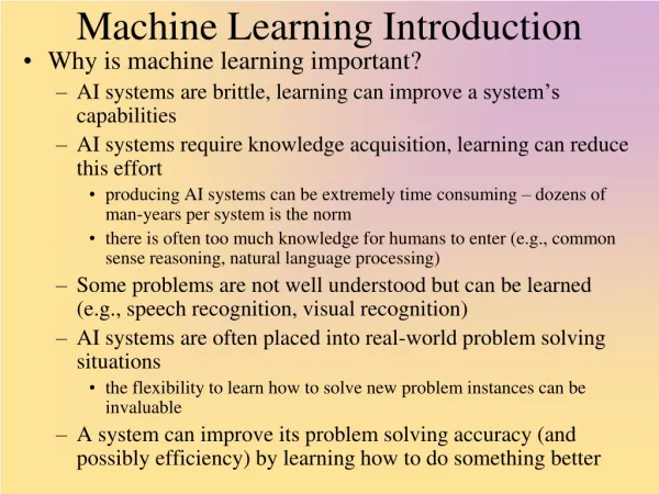
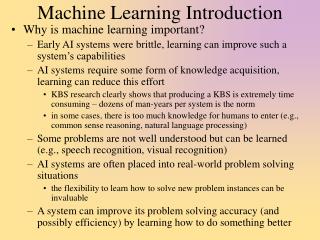
1. Machine Learning Introduction • Why is machine learning important? • Early AI systems were brittle, learning can improve such a system’s capabilities • AI systems require some form of knowledge acquisition, learning can reduce this effort • KBS research clearly shows that producing a KBS is extremely time consuming – dozens of man-years per system is the norm • in some cases, there is too much knowledge for humans to enter (e.g., common sense reasoning, natural language processing) • Some problems are not well understood but can be learned (e.g., speech recognition, visual recognition) • AI systems are often placed into real-world problem solving situations • the flexibility to learn how to solve new problem instances can be invaluable • A system can improve its problem solving accuracy (and possibly efficiency) by learning how to do something better

2. How Does Machine Learning Work? • Learning in general breaks down into one of two forms • Learning something new • no prior knowledge of the domain/concept so no previous representation of that knowledge • in ML, this requires adding new information to the knowledge base • Learning something new about something you already knew • add to the knowledge base or refine the knowledge base • modification of the previous representation • new classes, new features, new connections between them • Learning how to do something better, either more efficiently or with more accuracy • previous problem solving instance (case, chain of logic) can be “chunked” into a new rule (also called memoizing) • previous knowledge can be modified – typically this is a parameter adjustment like a weight or probability in a network that indicates that this was more or less important than previously thought

3. Types of Machine Learning • There are many ways to implement ML • Supervised vs. Unsupervised vs. Reinforcement • is there a “teacher” that rewards/punishes right/wrong answers? • Symbolic vs. Subsymbolic vs. Evolutionary • at what level is the representation? • subsymbolic is the fancy name for neural networks • evolutionary learning is actually a subtype of symbolic learning • Knowledge acquisition vs. Learning through problem solving vs. Explanation-based learning vs. Analogy • We can also focus on what is being learned • Learning functions • Learning rules • Parameter adjustment • Learning classifications • these are not mutually exclusive, for instance learning classification is often done by parameter adjustment

4. The idea behind supervised learning is that the learning system is offered examples The system uses what it already knows to respond to an input (if the system has yet to learn, initial values are randomly assigned) If correct, the system strengthens the components that led to the right answer If incorrect, the system weakens the components that led to the wrong answer This is performed for each item in the training set Repeat some number of iterations or until the system “converges” to an answer Below, we see that learning is actually a search problem The system is searching for the representation that will allow it to respond correctly to every (or most) instance in the training set There could be many “correct” solutions Some of these will also allow the system to respond correctly to most instances in the testing set Supervised Learning

5. Forms of Supervised Learning • Most ML is some form of learning a function • F(x) = y where x is the input (typically comprised of (x1, x2, …, xn) for some n-dimensional space, and y is the output • This form of learning typically breaks down into one of two forms: • classification – the training items are mapped to distinct elements of a set • regression – the training items are mapped to continuous values • In supervised learning, we have a training set of {x, y} pairs • Use the training set to “teach” the ML system • Many different approaches have been developed • neural networks using backpropagation • HMM • Bayesian networks • decision trees • clustering • Usually, once the system is trained, another data set (the test set) is run on the system to see how it performs • There is a danger in this approach, overtraining the system means that it learns the training set too well – it overfits to the training set such that it performs poorly on the test set

6. Learning a Function • One of the most basic ideas in learning is to provide examples of input/output and have the system learn the function • The system will not learn, say f(x1, x2) = x12 + 3x2 – 5 but instead will learn how to map f(xi, xj) to an output (hopefully reliably) • The function will be learned only approximately based on how useful the training set is and the specific type of learning algorithm applied Consider learning the function that fits the data points plotted to the left – there are many functions that might fit – which one is correct? Do we need to find a precise fit? If not, how much error should we allow?

7. Perceptrons • Earliest form of neural network • given a series of input/output pairs, identify the linear separability (a hyper-plane) • e.g., a line in 2-d, a plane in 3-d • If the data points are linearly separable, the perceptron learning algorithm is guaranteed to find it • many functions, such as XOR, are not linearly separable, in which case perceptrons fail Think of the points as items that are either in a given class or not, the perceptron learns to classify the items An n-input perceptron computes Weights are adjusted during learning to improve the perceptron’s performance – this amounts to learning the function that separates the “ins” from the “outs”

8. Another approach is based on the statistical method of regression analysis Here, the strategy is to identify the coefficients (such as a, b below) to fit the equation below, given the data set of <x, y> values e is some random element we need to expand on this to be an n-dimensional formula since our data will consist of elements X = {x1, x2, x3, …, xn}, and y There are a variety of ways to do regression including applying using some sort of distribution (e.g., Gaussian), applying the method of least squares, applying Bayesian probabilities, etc note: neural networks are a form of non-linear regression Linear Regression y = α + βx + e

9. Classifiers • The more common form of supervised learning is that of a classifier – the goal is to learn how to classify the data • f(x) = y means that x describes some input and y is its proper category (again x is actually {x1, x2, …, xn}) • Much of ML has revolved around classifiers • Naïve bayesian classifiers • Neural networks • K nearest neighbors • Boosting • Induction • version spaces • decision trees • inductive logic programming • Some of these forms of classifiers are used heavily in data mining, so we will hold off on discussion those until the next lecture (K nearest neighbors, boosting, decision trees) • We will skip version spaces and inductive logic programming as they are not as common today, but you might investigate them on your own

10. Bayesian Learning • Recall to apply Bayesian probabilities, we must either • have an enormous number of evidential hypotheses • or must assume that evidence are independent • The Naïve Bayesian Classifier takes the latter assumption • thus, it is known as naïve • p(C | e1, e2, e3) = P(C | e1) * P(C | e2) * P(C | e3) • rather than the more complex chain of probabilities that we saw previously • We can learn the prior and evidential probabilities by counting occurrences of evidence and hypotheses amongst the data in the training set • P(A | B) = # of times that A & B both appear in the training set / # of times that B appears in the training set • P(A) = # of times that A appears / size of the training set • in case any of these values appears 0 times, we might want to “smooth” the probability so that no conditional probability would ever be 0.0 • smoothing is done by adding some “hallucinated values” to both the numerator and denominator based on the size of the training set and some pre-established constant

11. Consider that I want to train a NBC on whether a particular text-based article is one that I would like to read Given a set of training articles, mark each as “yes” or “no” Create the following probabilities: P(wordi | yes) = probability that word i appears in an article i want to read P(wordi | no) = probability that word i appears in an article i do not want to read P(wordi) = probability that word i appears in an article this is known as the “bag of words” approach Now, given an article, compute P(yes | words) and P(no | words) where words = worda, wordb, wordc, … for each unique word in the article We can enhance this strategy by removing common words using phrases making sure that the bag contains important words Example Accuracy of the NBC given training set of size 0-10000

12. Rather than assuming evidential independence, we might prefer Bayesian nets We cannot learn (compute) the complex probabilities in a Bayesian network e.g., P(A | B & C & ~D What we can do, given these probabilities (or estimates), is learn the proper (best) structure for the Bayesian net this is done by taking our original network, making some minor change(s) to it, computing the result’s probability, and selecting the network with the highest probability for that result For instance, in the figure to the right, we want to know P(T | …) We compute that probability on several versions of the Bayesian net and select the network that provides the highest resulting probability in which T was found to be true (likely) Learning in Bayesian Networks

13. After proving perceptrons could not learn XOR, research into connectionism died for about 15 years A new learning algorithm, backpropagation, and a new type of layered network, the Artificial Neural Network, led to a revised interest in connectionism To the right is a multi-layered ANN I inputs some (0 or more) intermediate levels known as hidden layers O outputs Each layer is completely connected to the next layer Each edge has its own weight The goal of the backprop algorithm is to train the ANN to learn proper weights Introduction to Neural Networks

14. First – feed forward the input most NN use a sigmoid function to compute the output of a given node but otherwise, it is like computing the result of a perceptron node Determine the error (if any) by examining each output node and comparing the value to the expected value from the training set Backpropagate the error from the output nodes to the hidden layer nodes (formula for weight adjustment on the next slide) Continue to backpropagate the error to the previous level (another hidden layer or the input) note that since we don’t know what a given hidden layer node was supposed to be, we can’t directly compute an error here, we have to therefore modify our formula for adjusting the weight (again, see the next slide) Repeat the learning algorithm on the next training set item Repeat the entire training set until the network converges (weights change less than some D) NN Supervised Learning

15. How to Adjust Weights • For the weights connecting the hidden layer to the output, we adjust a weight wij as follows • wij = wij + sf * oj * (1 – oj) * (ej - oj) * i • sf is the scaling factor – this controls how quickly the network learns • oj is the output value of node j • ej is the expected value for output node j (as dictated by the training set item) • i is the input value • We do not know ej for the hidden layer nodes, so we have to revise the formula to adjust the weights between hidden layer a and hidden layer b, or between the input layer and the hidden layer • wij = wij + sf * oi * (1 – oi) * Sum (wk * vk) * i • wk is the weight connecting this node to node k in the next layer and vk is the value that node k provided during the feed-forward part of the algorithm

16. Learning Example Assume an input = <10, 30, 20> and expected output is <1, 0> from our training set. Use a scaling factor of 0.1. Recall computing output uses the sigmoid function below Part 1: Feed forward  H1 receives 7, H2 receives -5 H1 outputs = .9990, H2 outputs .0067 O1 receives 1.0996, O2 receives 3.1047 O1 outputs .7501, O2 outputs .9571

17. Example Continued Part 2: Compute Error at Output  O1 should be 1.0, O2 should be 0.0 • Part 3: Compute Error for Hidden Units: • Back prop to H1: (w11*δ01) + (w12*δO2) = • (1.1*0.0469)+(3.1*-0.0394) = -0.0706 • Compute H1’s error (multiply by h1(E)(1-h1(E)): • -0.0706 * (0.999 * (1-0.999)) = 0.0000705 = δH1 • Back prop to H2: (w21*δ01) + (w22*δO2) = • (0.1*0.0469)+(1.17*-0.0394) = -0.0414 • Compute H2’s error (multiply by h2(E)(1-h2(E)): • -0.0414 * (0.067 * (1-0.067)) = -0.00259= δH2

18. Example Continued Part 4: Adjust weights as new weight = old weight + scaling factor * error

19. Over or Under Training • The scaling factor controls how quickly the network can learn so why not make it a large value? • What the NN is actually doing is performing a task called gradient descent • weights are adjusted based on the derivative of the cost function • the learning algorithm is searching for the absolute minimum value, however because we are moving in small leaps, we might get stuck in a local minima • a local minima may learn the training set well, but not the testing set • So we control just how well the NN learns to classify the domain by • the scaling factor • the number of epochs • the training data set • But also impacting this is the structure and size of the network (which also impacts the number of epochs that it might take to train the network)

20. What a Neural Network Learns • There has been some confusion regarding what a NN can do and what it learns • The weights that a NN learns is a form of distributed representation – more specifically a distributed statistical model of what features are important for a given class • Aside from the input and output nodes, the hidden layer nodes do not represent any single thing but instead, groups of them represent intermediate concepts in the domain/problem being learned The facial recognition NN (on the right) has learned to recognize what direction a face is turned: up, right, left or straight). The hidden layer’s three nodes, when analyzed, are storing the pixels that make up the three rough images of a face turned in one of the directions

21. Problems with NNs • In terms of learning, NNs surpass most of the previously mentioned methods because they learn via non-linear regression • A NN might be stuck in a local minima resulting in excellent performance on the training set but poor performance on the test set • The number of epochs (iterations through the training set) is extremely random • it might take a few dozen epochs, in other cases, a million epochs • There is no way to predict, given the structure of a network, how well or quickly it will learn • NNs are not understandable by us, so we can’t really tell what the NN has learned or how the information is represented • NNs cannot generate explanations • NNs do poorly in knowledge-intensive problems (e.g., diagnosis) but very well in some recognition problems (e.g., OCR) • NNs have a fixed sized input so problems that deal with temporal issues (e.g., speech rec) perform problematically, but recurrent NNs are one way to possibly get around this problem

22. Avoiding Some of These Problems To avoid getting stuck in a local minima, one strategy is to use an additional factor called momentum which in effect changes the scaling factor over time One form of this is called simulated annealing To avoid over fitting the training set, do not use accuracy on the training set, instead every so often, test the testing set and use the accuracy on that set to judge convergence

23. HMM Learning • Known as the EM algorithm or Baum-Welch algorithm • Use one training set item with observations o1, o2, …, on • Work through the HMM, one observation at a time • Once you have “fed forward” this example • for each time interval t and each state transition from i at time t to j at time t+1, compute the estimator probability of transitions from i to j • at(i) * aij * bj(Ot+1) * bt+1(j) • Where at+1(i) = S (at(j)*aji) * bi(Ot+1) • bt(j) = S bt+1(i) * aij * bj(Ot+1) • aij is the transition from i to j • and bi(Ot) is the output probability, which is the probability of observable Ot being seen at state I • Now modify each transition probability aij and output probability bi(Ot) as follows • New aij = estimator probability from i to j / number of transitions out of i • New bi(Ot) = at(i) * bt(i) / expected number of times in j • When done with this iteration, replace the old transition probabilities with the new probabilities and repeat with the next training set example until either the HMM converges, or you have depleted the examples

24. Genetic Algorithms • Learning through manipulation of a feature space • The state is a vector representing features • binary vector - feature is present or absent • multi-valued vector - features represented by a discrete or continuous value • Supervised learning requiring a method of determining how good a given feature vector is • learning is viewed as a search problem: what is the ideal or optimal vector • Natural selection techniques will (hopefully) improve the performance of the search during successive iterations (called generations) • this form of learning can be used to learn recognition knowledge, control knowledge, planning/design knowledge, diagnostic knowledge • The “genetics” come in by considering that the vector is a chromosome which is mutated by various random operations, and then evaluated – the most fit chromosomes survive to become parents for the next generation

25. General Procedure for GAs • Repeat the following until either you have exceeded the number of stated generations or you have a vector that is found suitable • Start with a population of parent vectors • Breed children through mutation operations • Apply the fitness function to the children • Select those children which will become parents of the next generation • Decisions: • What is the fitness function? Is there a reasonable one available? • What mutation operations should be applied and how randomly? Should children be very similar to the parents or highly different? • How many children should be selected for the next generation? How many children should be produced by the parents? • How is selection going to take place?

26. Fitness and Selection • Unlike other forms of supervised learning where feedback is a previously known classification or value, here, the feedback for the worth of a vector is in the form of a fitness function • given a vector V, apply the function f(V) • use this value to determine this vector’s worth towards the next generation • a vector that is highly rated may be selected in forming the next generation of vectors whereas a vector that is lowly rated will probably not be used (unless randomly selected) • How do you determine which vectors to alter/mutate? • Fitness Ranking - use a fitness function to select the best available vector (or vectors) and use it (them) • Rank Method - use the fitness function but do not select the “best”, use probabilities instead • Random Selection - in addition to the top vector(s), some approaches randomly select some number of vectors from the remaining, lesser ranked ones • Diversity - determine which vectors are the most diverse from the top ranked one(s) and select it (them)

27. Mutation and Selection Mechanisms • Standard mutation methods are • inversion – moving around values in a vector • If p1 = {1, 2, 3, 4, 5, 6}, then this might result in {1, 5, 4, 3, 2, 6} • mutation – changing a feature’s value to another value • crossover (requires two chromosomes) – randomly swap some portion of the two vectors • If p1 = {5, 4, 3, 2, 6, 1} and p2 = {1, 6, 2, 3, 4, 5}, crossover may yield the two children {5, 4, 2, 3, 4, 1} and {1, 6, 3, 2, 6, 5} • How do you determine which vectors to alter/mutate? • Fitness ranking – select the best available vectors • Rank Method – rank the vectors as scored by the fitness function and then use a probabilistic mechanism for selection • if v1 is .5, v2 if .3 and v3 is .15 and v4 is .05, then v1 has a 50% chance of being selected, v2 has a 30% chance, v3 has a 15% chance and v4 a 5% chance • Random Selection – select the top vector(s) and select the remainder by random selection • Diversity – select the top vector(s) and then select the remainder by finding the most diverse from the ones already selected

28. This form of learning is most commonly applied to programming code unlike the GA approach, here the representation is some dynamic structure, commonly a tree the process of inversion, mutation or crossover is applied Since trees are formed out of syntactic parses of programs, we can manipulate a program using this approach notice that by randomly manipulating a program, it may no longer be syntactically valid however if we just use crossover, the result will hopefully remain syntactically valid (why?) What kind of fitness function might be used? Genetic Programming

29. Other Forms of Learning • Reinforcement learning • A variation on supervised learning – a learner must determine what action to take in a given situation that maximizes its reward – it does this through trial and error rather than through training examples • reinforcement learning is not a new learning technique but rather a type of problem which can be solved by any of a number of techniques including those already seen (NNs, HMMs, • Unsupervised learning • No training set, no feedback, a form of discovery • Commonly uses either a Bayesian inference to produce probabilities, or a statistical approach and clustering to produce class descriptions • mostly a topic for data mining, also sometimes referred to as discovery

30. Knowledge-based Learning • Back in the 1970s, machine learning mostly revolved around learning new concepts in a knowledge base • Version spaces – offering positive and negative examples of a class to learn the features that distinguish items that are in versus out of the class, see for example • http://www.site.uottawa.ca/~nat/Courses/CSI5387/ML_Lecture_2.ppt • http://www.cs.cf.ac.uk/Dave/AI2/node146.html • Explanation based learning – given a KB, offer one or more examples of a concept and have the system add representations that fit the new concepts being learned – a commonly sited example is to add to a chess program’s capability by understanding the strategy of a fork, see for example • http://www.cs.cf.ac.uk/Dave/AI2/node148.html#SECTION000162000000000000000 • Analogy – taking a model in one domain and applying it to another domain, often done through case based reasoning • Discovery – finding patterns in data, what we now call data mining, one early example was pioneered in a system called BACON that analyzed data to find laws (which also reasoned using analogy) • it was able to infer Kepler’s third law, Ohm’s law, Joule’s law, and the conservation of momentum by analyzing data