Queueing Theory (Delay Models)
Queueing Theory (Delay Models). Introduction. Total delay of the i-th customer in the system T i = W i + τ i N(t) : the number of customers in the system N q (t) : the number of customers in the queue N s (t) : the number of customers in the service

Queueing Theory (Delay Models)
E N D
Presentation Transcript
Total delay of the i-th customer in the system Ti = Wi + τi • N(t) : the number of customers in the system • Nq (t) : the number of customers in the queue • Ns (t) : the number of customers in the service • N : the avg number of customers in the queue • τ : the service time
T : the total delay in the system • λ: the customer arrival rate [#/sec]
Little’s Theorem E[N] = λE[T] • Number of customer in the system at t N(t)=A(t)-D(t) where • D(t) : the number of customer departures up to time t • A(t) : the number of customer arrivals up to time t
Poisson Process • The interarrival probability density function • mean: 1/λ, variance: 1/λ2 • for every t, δ≥0 where
Poisson Process • Characteristics of the Poisson process • Interarrival times are independent and exponentially distributed • If t n denotes the n-th arrival time and the interval τn = t n+1- t n , the probability distribution is
Sum of Poisson Random Variables • Xi , i =1,2,…,n, are independent RVs • Xi follows Poisson distribution with parameter li • Partial sum defined as: • Sn follows Poisson distribution with parameter l
Sampling a Poisson Variable • X follows Poisson distribution with parameter l • Each of the X arrivals is of type i with probability pi, i =1,2,…,n, independently of other arrivals;p1+ p2 +…+ pn = 1 • Xi denotes the number of type i arrivals • X1, X2,…Xn are independent • Xi follows Poisson distribution with parameter li= lpi
Merging & Splitting Poisson Processes l1 lp • A1,…, Ak independent Poisson processes with rates l1,…, lk • Merged in a single processA= A1+…+ Ak • A is Poisson process with rate l= l1+…+ lk p l l1+ l2 1-p l2 l(1-p) • A: Poisson processes with rate l • Split into processes A1 and A2 independently, with probabilities p and 1-p respectively • A1 is Poisson with rate l1= lpA2 is Poisson with rate l2= l(1-p)
Poisson Variable • mean • variance • Memoryless property (if exponentially distributed)
Review of Markov chain theory • Discrete time Markov chains • discrete time stochastic process {Xn |n=0,1,2,..} taking values from the set of nonnegative integers • Markov chain if • where
Markov chain • Markov chain formulation • Consider a discrete time MC where Nk is the number of customers at time k and N(t) is the number of customers at time t • probabilities where the arrival and departure processes are independent
Review of Markov chain theory • The transition probability matrix • n-step transition probabilities
Review of Markov chain theory • Chapman-Kolmogorov equations • detailed balance equations for birth-death systems (in steady state)
2/2 -11 2/2 1-2/2 1 2/2 Example 0 1 P0=(2-2)/(2-2(1-1)) the throuput= P0 *P(s=0| P0)*0+ P0 *P(s=1| P0)*1+ P0 *P(s=2| P0 )*2+ P1 *P(s=0| P1)*0+ P1 *P(s=1| P1)*1+ P1 *P(s=2| P1)*2
Continuous time Markov chains • {X(t)| t≥0} taking nonnegative integer values • υi : the transition rate from state i • qij : the transition rate from state i to j qij = υi Pij • the steady state occupancy probability of state j • Analog of detailed balance equations for DTMC
Birth-And-Death Process Queueing Theory
Birth-And-Death Process(cont.) • Equation Expressing This: State Rate In = Rate Out 0 m1P1 = l0P0 1 l0P0 + m2P2 = (l1 + m1) P1 2 l1P1 + m3P3 = (l2 + m2) P2 .... ................... N-1 lN-2PN-2 + mNPN = (lN-1 + mN-1) PN-1 N lN-1PN-1 + mN+1PN+1 = (lN + mN) PN .... ................... Queueing Theory
Birth-And-Death Process(cont.) • Finding Steady State Process: State 0: P1 = (l0 / m1) P0 1: P2 = (l1 / m2) P1 + (m1P1 - l0P0) / m2 = (l1 / m2) P1 + (m1P1 - m1P1) / m2 = (l1 / m2) P1 = Queueing Theory
Birth-And-Death Process(cont.) • Finding Steady State Process(cont.): State n-1: Pn = (ln-1 / mn) Pn-1 + (mn-1Pn-1- ln-2Pn-2) / mn = (ln-1 / mn) Pn-1 + (mn-1Pn-1- mn-1Pn-1) / mn = (ln-1 / mn) Pn-1 Queueing Theory
Birth-And-Death Process(cont.) • Finding Steady State Process(cont.): N: Pn+1 = (ln / mn+1) Pn+ (mnPn - ln-1Pn-1) / mn+1 = (ln / mn+1) Pn To Simplify: Let C = (ln-1ln-2 .... l0) / (mn mn-1 ......... m1) Then Pn = Cn P0 , N = 1, 2, .... Queueing Theory
M/M/1 queueing system • Arrival statistics: stochastic process taking nonnegative integer values is called a Poisson process with rate λ if • A(t) is a counting process representing the total number of arrivals from 0 to t • arrivals are independent • probability distribution function
M/M/1 queueing system P[1 arrival and no departure in δ]= where the arrival and departure processes are independent
M/M/1 queueing system • Global balance equation
M/M/1 queueing system from Then • Average number of customers in the system
M/M/1 queueing system • Average delay per customer (waiting time + service time) by Little’s theorem • Average waiting time • Average number of customer in queue • Server utilization
M/M/1 queueing system • example 1/λ=4 ms, 1/μ=3 ms
תרגיל • קצב הגע למערכת הוא *n • קצב השרות הוא *n • א. שרטט את דיאגרמת המצבים • ב. מצא את הסתברויות הסטציונרות • ג. מצא את מספר הצרכנים הממוצע במערכת במצב היציב • ד. מצא את זמן ההשהייה הממוצע במערכת באמצעות משפט LITTLE
פתרון • א • ב
פתרון • ג • ד
תרגיל • צומת ברשת משתמש בשיטת הניתוב הבאה: כאשר חבילה מגיע אליו ללא תלות ביעדה הוא מפנה אותה לקו יצאה אםם התור לקו זה הוא ריק ולא נשלחת ברגע זה שום חבילה דרך קו זה. אחרת חבילה זו מופנת חבילה זו דרך כו אחר כלשהו. נניח כי שמופע ההודעות לצומת הוא פואסוני עם אורך החבילות מתפלג אקספוננצילי אם וכיבולת הקו היא C. א. איזה חלק מהחבילות מגעות דרך קו ההעדיף ? ב.אם הוחלט להצמיד תור לקו המהיר, מה אורכו המינימלי של התור כך שההסתברות שחבילה תשודרנה בקו זה תהיה לפחות 0.9 בהנחה ש ? (האם המערכת במצב יציב?)
פתרון א Message Length: Transmission Rate: Transmission Time: Service Rate:
פתרון • ב
M/M/1 Example I Traffic to a message switching center for one of the outgoing communication lines arrive in a random pattern at an average rate of 240 messages per minute. The line has a transmission rate of 800 characters per second. The message length distribution (including control characters) is approximately exponential with an average length of 176 characters. Calculate the following principal statistical measures of system performance, assuming that a very large number of message buffers are provided: Queueing Theory
M/M/1 Example I (cont.) • (a) Average number of messages in the system • (b) Average number of messages in the queue waiting to be transmitted. • (c) Average time a message spends in the system. • (d) Average time a message waits for transmission • (e) Probability that 10 or more messages are waiting to be transmitted. Queueing Theory
M/M/1 Example I (cont.) • E[s] = Average Message Length / Line Speed = {176 char/message} / {800 char/sec} = 0.22 sec/message or • m = 1 / 0.22 {message / sec} = 4.55 message / sec • l = 240 message / min = 4 message / sec • r = l E[s] = l / m = 0.88 Queueing Theory
M/M/1 Example I (cont.) • (a) N= r / (1 - r) = 7.33 (messages) • (b) Nq = r2 / (1 - r) = 6.45 (messages) • (c) W = E[s] / (1 - r) = 1.83 (sec) • (d) Wq = r× E[s] / (1 - r) = 1.61 (sec) • (e) P [11 or more messages in the system] = r11 = 0.245 Queueing Theory
M/M/1 Example II A branch office of a large engineering firm has one on-line terminal that is connected to a central computer system during the normal eight-hourworking day. Engineers, who work throughout the city, drive to the branch office to use the terminal to make routine calculations. Statistics collected over a period of time indicate that the arrival pattern of people at the branch office to use the terminal has a Poisson (random) distribution, with a mean of 10 people coming to use the terminal each day. The distribution of time spent by an engineer at a terminal is exponential, with a Queueing Theory
M/M/1 Example II (cont.) mean of 30 minutes. The branch office receives complains from the staff about the terminal service. It is reported that individuals often wait over an hour to use the terminal and it rarely takes less than an hour and a half in the office to complete a few calculations. The manager is puzzled because the statistics show that the terminal is in use only 5 hours out of 8, on the average. This level of utilization would not seem to justify the acquisition of another terminal. What insight can queueing theory provide? Queueing Theory
M/M/1 Example II (cont.) • {10 person / day}×{1 day / 8hr}×{1hr / 60 min} = 10 person / 480 min = 1 person / 48 min ==> l = 1 / 48 (person / min) • 30 minutes : 1 person = 1 (min) : 1/30 (person) ==> m = 1 / 30 (person / min) • r = l / m = {1/48} / {1/30} = 30 / 48 = 5 / 8 Queueing Theory
M/M/1 Example II (cont.) • Arrival Rate l = 1 / 48 (customer / min) • Server Utilization r = l / m = 5 / 8 = 0.625 • Probability of 2 or more customers in system P[N ³ 2] = r2 = 0.391 • Mean steady-state number in the system L = E[N] = r / (1 - r) = 1.667 • S.D. of number of customers in the system sN = sqrt(r) / (1 - r) = 2.108 Queueing Theory
M/M/1 Example II (cont.) • Mean time a customer spends in the system W = E[w] = E[s] / (1 - r) = 80 (min) • S.D. of time a customer spends in the system sw = E[w] = 80 (min) • Mean steady-state number of customers in queue Nq = r2 / (1 - r) = 1.04 • Mean steady-state queue length of nonempty Qs E[Nq | Nq > 0] = 1 / (1 - r) = 2.67 • Mean time in queue Wq = E[q] = r×E[s] / (1 - r) = 50 (min) Queueing Theory
M/M/1 Example II (cont.) • Mean time in queue for those who must wait E[q | q > 0] = E[w] = 80 (min) • 90th percentile of the time in queue pq(90) = E[w] ln (10 r) = 80 * 1.8326 = 146.6 (min) Queueing Theory
M/M/m, M/M/m/m, M/M/∞ • M/M/m (infinite buffer) • detailed balance equations in steady state
M/M/m where From