Strategy for Exploring Data
This guide covers essential strategies for exploring data, including plotting graphs, identifying patterns, calculating summaries, understanding density curves, normal distributions, standardizing observations, and more.

Strategy for Exploring Data
E N D
Presentation Transcript
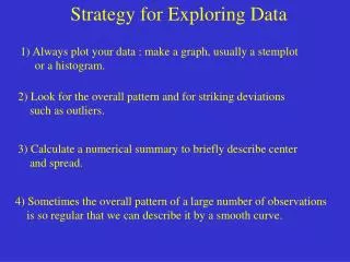
Strategy for Exploring Data 1) Always plot your data : make a graph, usually a stemplot or a histogram. 2) Look for the overall pattern and for striking deviations such as outliers. 3) Calculate a numerical summary to briefly describe center and spread. 4) Sometimes the overall pattern of a large number of observations is so regular that we can describe it by a smooth curve.
Density Curves A density curve is a curve that : 1) is always on or above the vertical axis, and 2) has area exactly 1 underneath it. A density curve describes the overall pattern of a distribution. The area under the curve and above any range of values is the relative frequency of all observations that fall in that range.
Normal and Skewed Curves Median Mean
Mean and Median of a Density Curve • The median of a density curve is the equal-areas point, the point • that divides the area under the curve in half. • The mean of a density curve is the balance point, at which the curve • would balance if made of solid material.
Normal Curves e 1 y = 2 -1 ( x - ) 2 2 Normal Curves are curves which are symmetric, unimodal, and bell shaped. • represents the mean • represents the • standard deviation • Equation for the curve :
Why are Normal Distributions important in stats? 1) Normal distributions are good descriptions for some distributions of real data. 2) Normal distributions are good to the results of many kinds of chance outcomes. 3) Many statistical inference procedures based on normal distributions work well for other roughly symmetric distributions.
The 68 - 95 - 99.7 Rule In the normal distribution with mean and standard deviation : • 68 % of the observations fall within of the mean • 95 % of the observations fall within2 of the mean • 99.7 % of the observations fall within3 of the mean
Normal Curve Example John collected data on the heights of women ages 18 to 24. He found that the distribution was roughly normal, with a mean of 64.5 inches and a standard deviation of 2.5 inches.
Normal Curve Example John collected data on the heights of women ages 18 to 24. He found that the distribution was roughly normal, with a mean of 64.5 inches and a standard deviation of 2.5 inches. Q1 : What percentage of these women were between the heights of 62 and 67 inches ? Q2 : What percentage of these women were between the heights of 59.5 and 69.5 inches ? Q3 : What percentage of these women were less than 64.5 inches tall ? Q4 : What percentage of these women were less than 67 inches tall ? Q5 : What percentage of these women were between the heights of 57 and 69.5 inches ?
Other Questions Q : What percentage of these women were between the heights of 60 and 70 inches ? Q : Who is considered more extraordinary, a 72 inch tall female or a 72 inch tall male ? Q : Who is considered more extraordinary, a 67 inch tall female or a 72 inch tall male ? Q : If you get a 26 on your ACT, and your neighbor gets a 1000 on their SAT, who did better? We can answer these questions by a “normalizing” technique.
“Normalizing” Data If we have two unrelated data sets, and they are both roughly normal, then we can perform a linear transformation on both data sets. This transformation will allow us to compare the data sets by examining how many standard deviations above or below the mean each score is. Example : Mike has an ACT score of 26 and Carol has an SAT score of 1250. Q : Who really has the better score ? A : Mike’s ACT score is 1.2 standard deviations above the mean, and Carol’s SAT score is 1.4 standard deviations above the mean. This means that Carol actually did better on her test than Mike!
Standardizing Observations x - z = 106 - 97 9 = = 6 6 If x is an observation from a roughly symmetric distribution that has mean and standard deviation , then the standard value of x is : Note: A standardized score is often called a z-score. Example : Women’s IQ’s have a symmetric distribution with a mean of 97 and a standard deviation of 6. What is the standard score for a woman with an IQ of 106 ? z = 1.5
Standardizing Observations x - z = 66 - 72 -6 = = 8 8 If x is an observation from a roughly symmetric distribution that has mean and standard deviation , then the standard value of x is : Note: A standardized score is often called a z-score. Example : Men’s IQ’s have a roughly symmetric distribution with a mean of 72 and a standard deviation of 8. What is the standard score for a man with an IQ of 66 ? z = - .75
Deep Thoughts 1) When we are “normalizing” our data set, we are really performing a linear transformation. This transformation will result in the data set still being normal. 2) If we start off with a distribution which is normal, with mean and standard deviation , (denoted by N( , ) ), then after we have standardized the data set, we will have a normal distribution, with mean 0 and standard deviation 1. (Denoted by N(0, 1) ).
Homework Section 1.3 79, 80, 82, 85, 86, 87