Ship-Board Flux Measurements from CalNex 2010: Insights from the Research Vessel Atlantis
This report details air-sea flux measurements conducted aboard the research vessel Atlantis during the California Air Quality Study (CalNex 2010). The study spanned from San Diego to San Francisco and included various meteorological observations and data sets, such as sensible and latent heat fluxes, solar radiation, precipitable water, and wind profiles. Special emphasis was placed on boundary layer conditions, analyzed through multiple radiosonde launches and Doppler cloud radar measurements. Key findings cover the diverse meteorological conditions experienced in both coastal and open ocean regions.

Ship-Board Flux Measurements from CalNex 2010: Insights from the Research Vessel Atlantis
E N D
Presentation Transcript
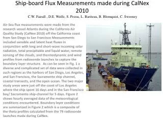
Ship-board Flux Measurements made during CalNex 2010 C.W. Fairall , D.E. Wolfe, S. Pezoa, L. Bariteau, B. Blomquist, C. Sweeney Air-Sea flux measurements were made from the research vessel Atlantis during the California Air Quality Study (CalNex 2010) off the California coast from San Diego to San Francisco Measurements included sensible and latent heat fluxes in conjunction with long and short-wave incoming solar radiation, total precipitable and liquid water, remote sensing of the clouds, and thermodynamic and wind profiles from radiosonde launches to capture the boundary layer structure. As can be seen in Fig. 1 a diverse and complicated set of data were collected in such regions as the harbors of San Diego, Los Angeles, and San Francisco, the Sacramento ship channel, coastal transects, and the open ocean. The two major study areas were just off the coast of Los Angeles where the ship spent 16 days and in the San Francisco bay/ Sacramento ship-channel for 5 days. Figure 2 shows hourly averaged data of the meteorological conditions encountered. Boundary layer conditions are summarized in Figure 2 which is a composite of the theta profiles calculated from the 79 radiosonde launches made during CalNex.
Sacramento RegionDateDOY A May 14 134 B May 15 – May 31 135-151 C June 2 152 D June 3-8 154-159 San Francisco D Monterey C Santa Barbara Los Angeles B San Diego A
CALNEX Wind Barb Plot C B A Each half pennant represents 5 knots (1 knot = 0.51 m/s) each whole pennant represents 10 knots; each flag represents 50 knots (which we should not see on that cruise). Max was ~30 knots.
Direct Turbulent Fluxes A C B
Column-Integrated Water Vapor (Precipitable Water) Region B Region D
Cloud Views Time-height cross section from 1 hour of data beginning at 1200 on May 5 from ESRL/PSD W-band cloud radar. The top panel is the radar reflectivity (dBZ); the middle panel is the mean Doppler velocity (m/s, positive down); the bottom panel is the Doppler width (m/s) of the return. Time series ofceilometercloudbase height for May 15.
Combined Ceilometer – Cloud Radar Time series of cloud properties for May 5, 2010. Upper panel: cloud top height (circle with solid line; ±1 standard deviation, dashed line) and cloud base height (diamonds with solid line; 1 standard deviation, dots). Lower panel: mean radar backscatter for the cloud/drizzle layer (circle with solid line) and mean droplet fall speed (x’s with solid line) multiplied by 10 (in m/s).
Time/height cross section of potential temperature Time series of BL/Mixing height (blue) and cloud base height (green)
Year Day 156 May 23, 2010 Cloud Radar Returns from Non Cloud Targets (Bugs, pollen, bird???) Upper panel: cloud top height from radar (circle with solid line; ±1 standard deviation, dashed line) and cloud base height from ceilometer (diamonds with solid line; 1 standard deviation, dots). Lower panel: mean radar backscatter for the cloud/drizzle layer (circle with solid line) and mean droplet fall speed (x’s with solid line) multiplied by 10 (in m/s).
Measurements of CO2 and CH4Blomquist/Huebert and Sweeney/McGillis Blomquist – Picarro CRD CO2 Sweeney – Picarro CRD CO2/CH4, H2O PSD – Licor7500 open path Sample Methane Signal Upper Panel – Detrended CO2 Picarro and Licor Lower Panel – Detrended Humidity – Blue; Temperature – Green;Vertical Velocity – Red;Ship Vertical Motion - Cyan