Enhancing Matrix Sampling with Iterative Row Sampling Techniques
This work explores matrix sketches and iterative algorithms for improving row sampling methods in data matrices. By utilizing better sampling techniques, we aim to enhance classification, clustering, and pattern identification in large datasets, where the number of rows significantly exceeds the number of columns. Our approach leverages statistical leverage scores and covariance matrices, resulting in effective computational methods that preserve essential data attributes while minimizing errors. This research provides insights into achieving superior sampling quality with manageable computational costs.

Enhancing Matrix Sampling with Iterative Row Sampling Techniques
E N D
Presentation Transcript
Iterative Row Sampling Richard Peng CMU MIT Joint work with Mu Li (CMU) and Gary Miller (CMU)
Outline • Matrix Sketches • Existence • Samples better samples • Iterative algorithms
Data • n-by-d matrix A, m entries • Columns: data • Rows: attributes A Goal: • Classification/ clustering • Identify patterns • Interpret new data
Linear Model • Can add/scale data points • x1: coefficients,combo: Ax x3A:,3 x2A:,2 Ax x1A:,1
Problem Interpret new data point b as combination of known ones Ax ?
Regression • Express as combination of current examples • Regression:minx ║Ax–b║ p • p=2: least squares • p=1: compressive sensing • ║x║2: Euclidean norm of x • ║x║1: sum of absolute values
Variants of Compressive Sensing • minx ║Ax-b║1 +║x║1 • minx║Ax-b║2 +║x║1 • minx ║x║1s.t.Ax=b • minx ║Ax║1s.t.Bx= y • minx║Ax-b║1 + ║Bx- y║1 All similar to minx║Ax-b║1
Simplified • minx║Ax–b║p= minx║[A,b] [x; -1]║p • Regression equivalent to min║Ax║p with one entry of x fixed x A b -1
‘Big’ Data Points • Each data point has many attributes • #rows (n) >> #columns (d) • Examples: • Genetic data • Time series (videos) • Reverse (d>>n) also common: images + SIFT A
Faster? A’ A Smaller, equivalent A’ Matrix sketch
Row Sampling • Pick some rows of A to be A’ • How to pick? Random A’ A
Shorter Equivalent • Find shorter A’ that preserves answer • |Ax|p≈1+ε|A’x|p for all x • Run algorithm on A’, same answer good for A A’ Simplified error notation ≈: a≈kb if there exists k1, k2s.t. k2/k1 ≤ k and k1a ≤ b ≤ k2 b
Outline • Matrix Sketches • How? Existence • Samples better samples • Iterative algorithms
Sketches Exist |Ax|p≈|A’x|p for all x • Linear sketches: A’=SA • [Drinealset al. `12]:Row sampling: one non-zero in each row of S • [Clarkson-Woodruff `12]:S = countSketch, one non-zero per column. A’
Sketches Exist Hidden: runtime costs, ε-2dependency
WHY is ≈d possible? |Ax|p≈|A’x|p for all x • ║Ax║22 = xTATAx • ATA: d-by-dmatrix • Any factorization (e.g. QR) of ATA suffices as A’
ATA A:,j1 A:,j2 • Covariance matrix • Dot product of all pairs of columns (data) • Covariance:cov(j1,j2) = ΣiAi,j1TAi,j2
Use of Covariance Matrix • Clustering: l2 distances of all pairs given by C • Kernel methods: all pair dot products suffice for many models. C=ATA C
Other Use of Covariance • Covariance of attributes used to tune parameters • Images + SIFT: many data points, few attributes. • http://www.image-net.org/: 14,197,122 images 1000 SIFT features C
How Expensive is this? • d2 dots of length n vectors • Total: O(nd2) • Faster: O(ndω-1) • Expensive: nd2 > nd > m C A
Equivalent View Of Sketches • Approximate covariance matrix: C’=(A’)TA’ • ║Ax║2≈║A’x║2 is the same as C ≈ C’ A’ C’
Application of Sketches • A’: n’ rows • d2 dots of length n’ vectors • Total cost: O(n’dω-1) A’ C’ A
Sketches in Input Sparsity Time • Need: cost of computing C’ < cost of computing C = ATA • 2 goals: • n’ small • A’ found efficiently A’ C’ A
Outline • Matrix Sketches • How? Existence • Samples better samples • Iterative algorithms
Previous Approaches A miracle happens • Go go poly(d) rows directly • Projection to obtain key info, or the sketch itself A’ A poly(d) m
Our Main Approach • Utilize the robustness of sketches, covariance matrices, and sampling • Iteratively reduce errors and sizes A” A’ A
Composing Sketches O(n’dlogd +dω) O(m) Total cost: O(m + n’dlogd + dω) = O(m + dω) A” A’ A n’ = d1+α n rows dlogd rows
Accumulation of Errors ║Ax║2 ≈kk’║A’x║2 ║A”x║2≈k’║A’x║2 ║Ax║2≈k║A”x║2 A” A’ A n’ = d1+α n rows dlogd rows
Accmulation of Errors • Final error: product of both errors • Dependency of error in cost: usually ε-2 or more for 1± ε error • [Avron & Toledo `11]: only final step needs to be accurate • Idea: compute sketches indirectly ║Ax║ 2≈kk’║A’x║2
Row Sampling • Pick some rows of A to be A’ • How to pick? Random A’ A
Are All Rows Equal? column with one entry one non-zero row A A |A[1;0;…;0]|p≠ 0
Row Sampling • τ’ : weights on rows distribution • Pick a number of rows independently from this distribution, rescale to form A’ A’ A
Matrix Chernoff Bounds • Sufficient property of τ’ • τ: statistical leverage scores • If τ' ≥ τ,║τ'║1logd (scaled) rows suffices for A’≈ A τ' A
Statistical Leverage Scores • Studied in stats since 70s • Importance of rows • leverage score of row i, Ai: • τi= Ai(ATA)-1AiT • Key fact: ║τ║1 = rank ≤ d • ║τ'║1logd = dlogd rows τ A
Computing Leverage scores • τi= Ai(ATA)-1AiT • = AiC-1AiT • ATA: covariance matrix, C • Given C-1, can compute each τiin O(d2) time • Total cost: O(nd2+dω)
Computing Leverage scores • τi= AiC-1AiT • =║AiC-1/2║22 • 2-norm of a vector, AiC-1/2 • rows in isotropic positions • Decorrelates columns
Aside: What is Leverage? Ai AiC-1/2 • Geometric view: • Rows define ‘energy’ directions. • Normalize so total energy is uniform • τi: norm of row i after normalizing
Aside: What is Leverage? • How to interpret statistical leverage scores? • Statistics ([Hoaglin-Welsh `78], [Chatterjee-Hadi `86]): • Influence on data set • Likelihood of outlier • Uniqueness of Row τ A
Aside: What is Leverage? • High Leverage Score: • Key attribute? • Outlier (measuring error)?
Aside: What is Leverage? • My current view (motivated by graph sparsification): • Sampling probabilities • Use them to find sketches τ A
Computing Leverage scores τi= ║AiC-1/2║22 • Only need τ' ≥ τ • Can use approximations after scaling them up • Error leads to larger ║τ'║1
Dimensionality Reduction x Gx ║x║22 ≈jl║Gx║22 • Johnson Lindenstrauss Transform • G: d-by-O(1/α) Gaussian • Errorjl = dα
Estimating Leverage scores τi=║AiC-1/2║22 ≈jl║AiC-1/2G║22 • G: d-by-O(1/α) Gaussian • C1/2G: d-by-O(1/α) • Cost: O(α ∙ nnz(Ai))total: O(α ∙ m + α ∙ d2logd)
Estimating Leverage scores τi=║AiC-1/2║ 22 ≈║AiC’-1/2║ 22 • C ≈k C’ gives ║C-1/2x║2≈k║C’-1/2x║2 • Using C’ as a preconditioner for C • Can also combine with JL
Estimating Leverage scores • τi’=║AiC’-1/2G║22 • ≈jl║AiC-1/2║22 • ≈jl∙kτi • (jl∙ k) ∙ τ’≥ τ • Total number of rows: • ║jl ∙ k ∙ τ’║1 ≤ jl ∙ k ∙║τ’║1 • ≤ k d1 + α
Estimating Leverage scores • (jl ∙ k) ∙ τ’≥ τ • ║jl∙ k ∙ τ’║1 ≤ jl ∙ k ∙ d1+α • Quality of A’ does not depend on quality of τ' • C ≈k C’ gives A’≈2A with O(kd1+α) rows in O(m + dω) time Some fixableissues when n >>>d
Size reduction A” C” A’ τ' • A” ≈O(1) A • C” ≈O(1) C • τ' ≈O(1) τ • A’ ≈O(1) A , O(d1+α logd) rows
High Error Setting A” C” A’ τ' • A” ≈k A • C” ≈k C • τ'≈k τ • A’ ≈O(1) A , O(kd1+α logd) rows