Efficient Iterative Sampling for Gaussian Distributions
340 likes | 448 Vues
This research article explores techniques for efficient iterative sampling of multivariate Gaussian distributions, providing advantages and disadvantages of various methods such as CG-Lanczos and Gibbs sampling. It discusses the convergence guarantees and trade-offs in computational complexity for large Gaussian distributions, introducing solutions for working with sparse precision matrices. The use of iterative methods like Chebyshev-Gibbs and Lanczos is emphasized, along with their applications in solving linear systems. The text also covers the relationship between solving Ax=b and sampling from Gaussian distributions using iterative techniques, illustrating how the CG-Lanczos method estimates solutions and eigenvectors of the covariance matrix. Examples and comparisons between different iterative sampling methods are presented, showcasing their accuracy and efficiency in generating samples from Gaussian distributions with arbitrary covariance or precision matrices. The article concludes with insights into maintaining orthogonal Krylov bases and geometric convergence properties of iterative samplers for Gaussian distributions.

Efficient Iterative Sampling for Gaussian Distributions
E N D
Presentation Transcript
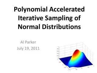
Polynomial Accelerated Iterative Sampling of Normal Distributions Al Parker July 19, 2011
Acknowledgements • Colin Fox, Physics, University of Otago • New Zealand Institute of Mathematics, University of Auckland • Center for Biofilm Engineering, , Bozeman
How to sample from a Gaussian N(µ,Σ)? • y = Σ1/2 z+ µ • ~ N(µ,Σ) • Sample z ~ N(0,I)
The problem • To generate a sample y = Σ1/2 z+ µ ~ N(µ,Σ), how to calculate the factorization Σ =Σ1/2(Σ1/2)T ? • Σ1/2 = WΛ1/2 by eigen-decomposition, 10/3n3 flops • Σ1/2 = C by Cholesky factorization, 1/3n3 flops • For LARGE Gaussians (n>105, eg in image analysis and global data sets), these factorizations are not possible • n3 is computationally TOO EXPENSIVE • storing an n x n matrix requires TOO MUCH MEMORY
Some solutions Work with sparse precision matrix Σ-1 models (Rue, 2001) Circulant embeddings (Gneiting et al, 2005) Iterative methods: • Advantages: • COST: n2 flops per iteration • MEMORY: Only vectors of size n x 1 need be stored • Disadvantages: • If the method runs for n iterations, then there is no cost savings over a direct method
What iterative samplers are available? Sampling y ~ N(0,A-1): Gibbs Chebyshev-Gibbs Lanczos Solving Ax=b: Gauss-Seidel Chebyshev-GS CG-Lanczos
What’s the link to Ax=b? Solving Ax=b is equivalent to minimizing an n-dimensional quadratic (when A is spd) A Gaussian is sufficiently specified by the same quadratic (with A= Σ-1and b=Aμ):
CG-Lanczos solver and sampler Schneider and Willsky, 2001 Parker and Fox, 2011 • CG-Lanczos estimates: • a solution to Ax=b • eigenvectors of A • in a k-dimensional Krylov space • CG sampler produces: • y ~ N(0, Σy ≈ A-1) • Ay ~ N(0, AΣyA ≈ A) • with accurate covariances in the same • k-dimensional Krylov space
CG-Lanczos solver in finite precision The CG-Lanczos search directions span a Krylov space much smaller than the full space of interest. CG is still guaranteed to find a solution to Ax = b … Lanczoseigensolver will only estimate a few of the eigenvectors of A … CG sampler produces y ~ N(0, Σy ≈ A-1) Ay ~ N(0, AΣyA ≈ A) with accurate covariances … … in the eigenspaces corresponding to the well separated eigenvalues of A that are contained in the k-dimensional Krylov space
Example: N(0,A) over a 1D domain A = eigenvalues of A Only 8 eigenvectors (corresponding to the 8 largest eigenvalues) are sampled (and estimated) by the CG sampler covariance matrix
Example: N(0,A) over a 1D domain Ay ~ N(0, A) Cholesky sample CG sample λ-(k+1) ≤ ||A - Var(AyCG)||2 ≤ λ -(k+1) + ε
Example: 104Laplacian over a 2D domain A(100:100) = A-1(100:100) = precision matrix covariance matrix
Example: 104Laplacian over a 2D domain eigenvalues of A-1 35 eigenvectors are sampled (and estimated) by the CG sampler.
Example: 104Laplacian over a 2D domain y ~ N(0, A-1) Cholesky sample CG sample trace(Var(yCG)) / trace(A-1) = 0.80
How about an iterative sampler from LARGE Gaussians that is guaranteed to converge for arbitrary covariance or precision matrices? Could apply re-orthogonalization to maintain an orthogonal Krylov basis, but this is expensive (Schneider and Willsky, 2001)
Gibbs: an iterative sampler Gibbs sampling from N(µ,Σ) starting from (0,0)
Gibbs: an iterative sampler of N(0,A) and N(0,A-1 ) Let A=Σ or A= Σ-1 • Split A into D=diag(A), L=lower(A), LT=upper(A) • Sample z ~ N(0,I) • Take conditional samples in each coordinate direction, so that a full sweep of all n coordinates is yk =-D-1 L yk - D-1 LT yk-1 + D-1/2 z yk converges in distribution geometrically to N(0,A-1) E(yk)= Gk E(y0) Var(yk) = A-1 - Gk (A-1 - Var(y0))GkT Aykconverges in distribution geometrically to N(0,A) Goodman and Sokal, 1989
Gauss-Siedel Linear Solve of Ax=b • Split A into D=diag(A), L=lower (A), LT=upper(A) • Minimize the quadratic f(x) in each coordinate direction, so that a full sweep of all n coordinates is • xk =-D-1 L xk - D-1 LT xk-1 + D-1 b xk converges geometrically A-1b (xk- A-1b) = Gk( x0 - A-1b) where ρ(G) < 1
Theorem: A Gibbs sampler is a Gauss Siedel linear solver Proof: • A Gibbs sampler is yk =-D-1 L yk - D-1 LT yk-1 + D-1/2 z • A Gauss-Siedel linear solve of Ax=b is xk =-D-1 L xk - D-1 LT xk-1 + D-1 b
Gauss Siedel is a Stationary Linear Solver • A Gauss-Siedel linear solve of Ax=b is xk =-D-1 L xk - D-1 LT xk-1 + D-1 b • Gauss Siedel can be written as M xk = N xk-1 + b where M = D + L and N = D - LT , A = M – N, the general form of a stationary linear solver
Stationary Samplers from Stationary Solvers • Solving Ax=b: • Split A=M-N, where M is invertible • Iterate Mxk = N xk-1 + b • xk A-1b if ρ(G=M-1N)< 1 Need to be able to easily solve M y = u Need to be able to easily sample ck-1 • Sampling from N(0,A) and N(0,A-1): • Split A=M-N, where M is invertible • Iterate Myk = N yk-1 + ck-1 • where ck-1 ~ N(0, MT + N) • yk N(0,A-1) if ρ(G=M-1N)< 1 • Ayk N(0,A) if ρ(G=M-1N)< 1
Theorem: Stat Linear Solver converges iffStat Sampler converges Proof: They have the same iteration operator G=M-1N: For linear solves: xk = Gxk-1 + M-1 b so that (xk- A-1b) = Gk( x0 - A-1b) For sampling G=M-1N: yk = Gyk-1 + M-1 ck-1 E(yk)= Gk E(y0) Var(yk) = A-1 - Gk (A-1 - Var(y0))GkT Proof for SOR given by Adler 1981; Barone and Frigessi, 1990; Amit and Grenander 1991. SSOR/REGS: Roberts and Sahu 1997.
Acceleration schemes for stationary linear solvers can be used to accelerate stationary samplers Polynomial acceleration of a stationary solver of Ax=b is 1. Split A = M - N 2.xk+1 = (1- vk) xk-1 + vkxk + vkuk M-1 (b-A xk) which replaces (xk- A-1b) = Gk(x0 - A-1b) = (I - (I - G))k(x0 - A-1b) with a different kth order polynomial with smaller spectral radius (xk- A-1b) = Pk(I-G)(x0 - A-1b)
Some polynomial accelerated linear solvers … xk+1 = (1- vk) xk-1 + vkxk + vkuk M-1 (b-A xk) Chebyshev-GS CG-Lanczos Gauss-Seidel vkand ukare functions of the 2 extreme eigenvalues of G vk , ukare functions of the residuals b-Axk vk = uk = 1
Some polynomial accelerated linear solvers … (xk- A-1b) = Pk(I-G)(x0 - A-1b) CG-Lanczos Gauss-Seidel Chebyshev-GS Pk(I-G) is the kth order Chebyshev polynomial (which has the smallest maximum between the two eigenvalues). Pk(I-G) = Gk Pk(I-G) is the kth order Lanczospolynomial
How to find polynomial accelerated samplers? yk+1 = (1- vk) yk-1 + vkyk + vkuk M-1 (ck -A yk) ck ~ N(0, (2-vk)/vk ( (2 – uk)/ ukM + N) Gibbs Chebyshev-Gibbs Lanczos vkand ukare functions of the 2 extreme eigenvalues of G vk,ukare functions of the residuals b-Axk vk = uk = 1
Convergence of polynomial accelerated samplers (A-1 - Var(yk))v = 0 (A - Var(Ayk))v = 0 for any Krylov vector v E(yk)=Pk(I-G)E(y0) Var(yk) = A-1 - Pk(I-G)(A-1 - Var(y0))Pk(I-G)T CG-Lanczos Gibbs Chebyshev-Gibbs Pk(I-G) is the kth order Chebyshev polynomial (which has the smallest maximum between the two eigenvalues). Pk(I-G) = Gk Pk(I-G) is the kth order Lanczospolynomial Theorem: The sampler converges if the solver converges Fox and Parker, 2011
Chebyshev accelerated Gibbs sampler of N(0, -1 ) in 100D Covariance matrix convergence ||A-1 – Var(yk)||2
Chebyshev accelerated Gibbs can be adapted to sample under positivity constraints
One extremely effective sampler for LARGE Gaussians Use a combination of the ideas presented: • Use the CG sampler to generate samples and estimates of the extreme eigenvalues of G. • Seed these samples and extreme eigenvalues into a Chebyshev accelerated SSOR sampler
Conclusions Common techniques from numerical linear algebra can be used to sample from Gaussians • Cholesky factorization (precise but expensive) • Any stationary linear solver can be used as a stationary sampler (inexpensive but with geometric convergence) • Polynomial accelerated Samplers • Chebyshev(precise and inexpensive) • CG (precise in a some eigenspaces and inexpensive)
