BIOINFORMATICS Multiple Sequences
BIOINFORMATICS Multiple Sequences. Mark Gerstein, Yale University gersteinlab.org/courses/452 (last edit in spring '11, not including in-class edits). Multiple Alignment Topics. Multiple Alignment Motifs Fast identification methods Profile Patterns Refinement via EM Gibbs Sampling HMMs

BIOINFORMATICS Multiple Sequences
E N D
Presentation Transcript
BIOINFORMATICSMultiple Sequences Mark Gerstein, Yale Universitygersteinlab.org/courses/452 (last edit in spring '11, not including in-class edits)
Multiple Alignment Topics • Multiple Alignment • Motifs • Fast identification methods • Profile Patterns • Refinement via EM • Gibbs Sampling • HMMs • Applications • Module DBs • Regression vs expression • Issues: site independence • BoCaTFBS
Multiple Sequence Alignments - Practically useful methods only since 1987 - Before 1987 they were constructed by hand - The basic problem: no dynamic programming approach can be used - First useful approach by D. Sankoff (1987) based on phylogenetics - One of the most essential tools in molecular biology It is widely used in: - Phylogenetic analysis - Prediction of protein secondary/tertiary structure - Finding diagnostic patterns to characterize protein families - Detecting new homologies between new genes and established sequence families (LEFT, adapted from Sonhammer et al. (1997). “Pfam,” Proteins 28:405-20. ABOVE, G Barton AMAS web page)
Progressive Multiple Alignments - Most multiple alignments based on this approach - Initial guess for a phylogenetic tree based on pairwise alignments - Built progressively starting with most closely related sequences - Follows branching order in phylogenetic tree - Sufficiently fast - Sensitive - Algorithmically heuristic, no mathematical property associated with the alignment - Biologically sound, it is common to derive alignments which are impossible to improve by eye (adapted from Sonhammer et al. (1997). “Pfam,” Proteins 28:405-20)
Ca28_HumanELSAHATPAFTAVLTSPLPASGMPVKFDRTLYNGHSGYNPATGIFTCPVGGVYYFAYHVHVKGTNVWVALYKNNVPATYTYDEYKKGYLDQASGGAVLQLRPNDQVWVQIPSDQANGLYSTEYIHSSFSGFLLCPTC1qb_HumanDYKATQKIAFSATRTINVPLRRDQTIRFDHVITNMNNNYEPRSGKFTCKVPGLYYFTYHASSRGNLCVNLMRGRERAQKVVTFCDYAYNTFQVTTGGMVLKLEQGENVFLQATDKNSLLGMEGANSIFSGFLLFPDCerb_HumanVRSGSAKVAFSAIRSTNHEPSEMSNRTMIIYFDQVLVNIGNNFDSERSTFIAPRKGIYSFNFHVVKVYNRQTIQVSLMLNGWPVISAFAGDQDVTREAASNGVLIQMEKGDRAYLKLERGNLMGGWKYSTFSGFLVFPLCOLE_LEPMA.264RGPKGPPGESVEQIRSAFSVGLFPSRSFPPPSLPVKFDKVFYNGEGHWDPTLNKFNVTYPGVYLFSYHITVRNRPVRAALVVNGVRKLRTRDSLYGQDIDQASNLALLHLTDGDQVWLETLRDWNGXYSSSEDDSTFSGFLLYPDTKKPTAMHP27_TAMAS.72GPPGPPGMTVNCHSKGTSAFAVKANELPPAPSQPVIFKEALHDAQGHFDLATGVFTCPVPGLYQFGFHIEAVQRAVKVSLMRNGTQVMEREAEAQDGYEHISGTAILQLGMEDRVWLENKLSQTDLERGTVQAVFSGFLIHENHSUPST2_1.95GIQGRKGEPGEGAYVYRSAFSVGLETYVTIPNMPIRFTKIFYNQQNHYDGSTGKFHCNIPGLYYFAYHITVYMKDVKVSLFKKDKAMLFTYDQYQENNVDQASGSVLLHLEVGDQVWLQVYGEGERNGLYADNDNDSTFTGFLLYHDTN2.HS27109_1ENALAPDFSKGSYRYAPMVAFFASHTYGMTIPGPILFNNLDVNYGASYTPRTGKFRIPYLGVYVFKYTIESFSAHISGFLVVDGIDKLAFESENINSEIHCDRVLTGDALLELNYGQEVWLRLAKGTIPAKFPPVTTFSGYLLYRT4.YQCC_BACSUVVHGWTPWQKISGFAHANIGTTGVQYLKKIDHTKIAFNRVIKDSHNAFDTKNNRFIAPNDGMYLIGASIYTLNYTSYINFHLKVYLNGKAYKTLHHVRGDFQEKDNGMNLGLNGNATVPMNKGDYVEIWCYCNYGGDETLKRAVDDKNGVFNFFD5.BSPBSXSE_25ADSGWTAWQKISGFAHANIGTTGRQALIKGENNKIKYNRIIKDSHKLFDTKNNRFVASHAGMHLVSASLYIENTERYSNFELYVYVNGTKYKLMNQFRMPTPSNNSDNEFNATVTGSVTVPLDAGDYVEIYVYVGYSGDVTRYVTDSNGALNYFDCa28_HumanELSAHATPAFTAVLTSPLPASGMPVKFDRTLYNGHSGYNPATGIFTCPVGGVYYFAYHVHVKGTNVWVALYKNNVPATYTYDEYKKGYLDQASGGAVLQLRPNDQVWVQIPSDQANGLYSTEYIHSSFSGFLLCPTC1qb_HumanDYKATQKIAFSATRTINVPLRRDQTIRFDHVITNMNNNYEPRSGKFTCKVPGLYYFTYHASSRGNLCVNLMRGRERAQKVVTFCDYAYNTFQVTTGGMVLKLEQGENVFLQATDKNSLLGMEGANSIFSGFLLFPDCerb_HumanVRSGSAKVAFSAIRSTNHEPSEMSNRTMIIYFDQVLVNIGNNFDSERSTFIAPRKGIYSFNFHVVKVYNRQTIQVSLMLNGWPVISAFAGDQDVTREAASNGVLIQMEKGDRAYLKLERGNLMGGWKYSTFSGFLVFPLCOLE_LEPMA.264RGPKGPPGESVEQIRSAFSVGLFPSRSFPPPSLPVKFDKVFYNGEGHWDPTLNKFNVTYPGVYLFSYHITVRNRPVRAALVVNGVRKLRTRDSLYGQDIDQASNLALLHLTDGDQVWLETLRDWNGXYSSSEDDSTFSGFLLYPDTKKPTAMHP27_TAMAS.72GPPGPPGMTVNCHSKGTSAFAVKANELPPAPSQPVIFKEALHDAQGHFDLATGVFTCPVPGLYQFGFHIEAVQRAVKVSLMRNGTQVMEREAEAQDGYEHISGTAILQLGMEDRVWLENKLSQTDLERGTVQAVFSGFLIHENHSUPST2_1.95GIQGRKGEPGEGAYVYRSAFSVGLETYVTIPNMPIRFTKIFYNQQNHYDGSTGKFHCNIPGLYYFAYHITVYMKDVKVSLFKKDKAMLFTYDQYQENNVDQASGSVLLHLEVGDQVWLQVYGEGERNGLYADNDNDSTFTGFLLYHDTN2.HS27109_1ENALAPDFSKGSYRYAPMVAFFASHTYGMTIPGPILFNNLDVNYGASYTPRTGKFRIPYLGVYVFKYTIESFSAHISGFLVVDGIDKLAFESENINSEIHCDRVLTGDALLELNYGQEVWLRLAKGTIPAKFPPVTTFSGYLLYRT4.YQCC_BACSUVVHGWTPWQKISGFAHANIGTTGVQYLKKIDHTKIAFNRVIKDSHNAFDTKNNRFIAPNDGMYLIGASIYTLNYTSYINFHLKVYLNGKAYKTLHHVRGDFQEKDNGMNLGLNGNATVPMNKGDYVEIWCYCNYGGDETLKRAVDDKNGVFNFFD5.BSPBSXSE_25ADSGWTAWQKISGFAHANIGTTGRQALIKGENNKIKYNRIIKDSHKLFDTKNNRFVASHAGMHLVSASLYIENTERYSNFELYVYVNGTKYKLMNQFRMPTPSNNSDNEFNATVTGSVTVPLDAGDYVEIYVYVGYSGDVTRYVTDSNGALNYFD C1Q - Example
MMCOL10A1_1.483 SGMPLVSANHGVTG-------MPVSAFTVILS--KAYPA---VGCPHPIYEILYNRQQHYCa1x_Chick ----------ALTG-------MPVSAFTVILS--KAYPG---ATVPIKFDKILYNRQQHYS15435 ----------GGPA-------YEMPAFTAELT--APFPP---VGGPVKFNKLLYNGRQNYCA18_MOUSE.597 HAYAGKKGKHGGPA-------YEMPAFTAELT--VPFPP---VGAPVKFDKLLYNGRQNYCa28_Human ----------ELSA-------HATPAFTAVLT--SPLPA---SGMPVKFDRTLYNGHSGYMM37222_1.98 ----GTPGRKGEPGE---AAYMYRSAFSVGLETRVTVP-----NVPIRFTKIFYNQQNHYCOLE_LEPMA.264 ------RGPKGPPGE---SVEQIRSAFSVGLFPSRSFPP---PSLPVKFDKVFYNGEGHWHP27_TAMAS.72 -------GPPGPPGMTVNCHSKGTSAFAVKAN--ELPPA---PSQPVIFKEALHDAQGHFS19018 ----------NIRD-------QPRPAFSAIRQ---NPMT---LGNVVIFDKVLTNQESPYC1qb_Mouse --------------D---YRATQKVAFSALRTINSPLR----PNQVIRFEKVITNANENYC1qb_Human --------------D---YKATQKIAFSATRTINVPLR----RDQTIRFDHVITNMNNNYCerb_Human --------------V---RSGSAKVAFSAIRSTNHEPSEMSNRTMIIYFDQVLVNIGNNF2.HS27109_1 ---ENALAPDFSKGS---YRYAPMVAFFASHTYGMTIP------GPILFNNLDVNYGASY .* . : : MMCOL10A1_1.483 DPRSGIFTCKIPGIYYFSYHVHVKGT--HVWVGLYKNGTP-TMYTY---DEYSKGYLDTACa1x_Chick DPRTGIFTCRIPGLYYFSYHVHAKGT--NVWVALYKNGSP-VMYTY---DEYQKGYLDQAS15435 NPQTGIFTCEVPGVYYFAYHVHCKGG--NVWVALFKNNEP-VMYTY---DEYKKGFLDQACA18_MOUSE.597 NPQTGIFTCEVPGVYYFAYHVHCKGG--NVWVALFKNNEP-MMYTY---DEYKKGFLDQACa28_Human NPATGIFTCPVGGVYYFAYHVHVKGT--NVWVALYKNNVP-ATYTY---DEYKKGYLDQAMM37222_1.98 DGSTGKFYCNIPGLYYFSYHITVYMK--DVKVSLFKKDKA-VLFTY---DQYQEKNVDQACOLE_LEPMA.264 DPTLNKFNVTYPGVYLFSYHITVRNR--PVRAALVVNGVR-KLRTR---DSLYGQDIDQAHP27_TAMAS.72 DLATGVFTCPVPGLYQFGFHIEAVQR--AVKVSLMRNGTQ-VMERE---AEAQDG-YEHIS19018 QNHTGRFICAVPGFYYFNFQVISKWD--LCLFIKSSSGGQ-PRDSLSFSNTNNKGLFQVLC1qb_Mouse EPRNGKFTCKVPGLYYFTYHASSRGN---LCVNLVRGRDRDSMQKVVTFCDYAQNTFQVTC1qb_Human EPRSGKFTCKVPGLYYFTYHASSRGN---LCVNLMRGRER--AQKVVTFCDYAYNTFQVTCerb_Human DSERSTFIAPRKGIYSFNFHVVKVYNRQTIQVSLMLNGWP----VISAFAGDQDVTREAA2.HS27109_1 TPRTGKFRIPYLGVYVFKYTIESFSA--HISGFLVVDGIDKLAFESEN-INSEIHCDRVL . * * * * : MMCOL10A1_1.483 SGSAIMELTENDQVWLQLPNA-ESNGLYSSEYVHSSFSGFLVAPM-------Ca1x_Chick SGSAVIDLMENDQVWLQLPNS-ESNGLYSSEYVHSSFSGFLFAQI-------S15435 SGSAVLLLRPGDRVFLQMPSE-QAAGLYAGQYVHSSFSGYLLYPM-------CA18_MOUSE.597 SGSAVLLLRPGDQVFLQNPFE-QAAGLYAGQYVHSSFSGYLLYPM-------Ca28_Human SGGAVLQLRPNDQVWVQIPSD-QANGLYSTEYIHSSFSGFLLCPT-------MM37222_1.98 SGSVLLHLEVGDQVWLQVYGDGDHNGLYADNVNDSTFTGFLLYHDTN-----COLE_LEPMA.264 SNLALLHLTDGDQVWLETLR--DWNGXYSSSEDDSTFSGFLLYPDTKKPTAMHP27_TAMAS.72 SGTAILQLGMEDRVWLENKL--SQTDLERG-TVQAVFSGFLIHEN-------S19018 AGGTVLQLRRGDEVWIEKDP--AKGRIYQGTEADSIFSGFLIFPS-------C1qb_Mouse TGGVVLKLEQEEVVHLQATD---KNSLLGIEGANSIFTGFLLFPD-------C1qb_Human TGGMVLKLEQGENVFLQATD---KNSLLGMEGANSIFSGFLLFPD-------Cerb_Human SNGVLIQMEKGDRAYLKLER---GN-LMGG-WKYSTFSGFLVFPL-------2.HS27109_1 TGDALLELNYGQEVWLRLAK----GTIPAKFPPVTTFSGYLLYRT------- . :: : : . : * *:*. Clustal Alignment
Problems with Progressive Alignments - Local Minimum Problem - Parameter Choice Problem 1. Local Minimum Problem - It stems from greedy nature of alignment (mistakes made early in alignment cannot be corrected later) - A better tree gives a better alignment (UPGMA neighbour-joining tree method) 2. Parameter Choice Problem • - It stems from using just one set of parameters (and hoping that they will do for all)
Fuse multiple alignment into: • - Motif: a short signature pattern identified in the conserved region of the multiple alignment • - Profile: frequency of each amino acid at each position is estimated • HMM: Hidden Markov Model, a generalized profile in rigorous mathematical terms Profiles MotifsHMMs Core Can get more sensitive searches with these multiple alignment representations (Run the profile against the DB.)
Multiple Alignment motifs
Examples of when you would want to find motifs -- Finding TF-binding sequences • ChIP-on-chip or ChIP-seq: Immunoprecipitate DNA-TF complexes, then either hybridize them to a microarray chip or sequence them. • List promoter regions of co-regulated genes. • SELEX: Systematic Evolution of Ligands by Exponential Enrichment (or in vitro selection). A library of random oligonucleotides are bound to a purified protein, then the bound ones are identified. [Adapted from C Bruce, CBB752 '09]
Two problems in motif analysis • Given a collection of binding sites, develop a representation of those sites that can be used to search new sites and reliably predict where additional binding sites occur. • Given a set of sequences known to contain binding sites for a common factor, but not knowing where the sites are, discover the location of the sites in each sequence and a representation of the protein. [Adapted from C Bruce, CBB752 '09]
Two classes of motif discovery algorithms • Multiple alignment methods. • Return PWM; use local search techniques such as Gibbs sampling or EM • Deterministic combinatorial algorithms based on word frequency counts. • Search for various sized sequences exhaustively and evaluate significance. [Adapted from C Bruce, CBB752 '09]
- several proteins are grouped together by similarity searches - they share a conserved motif - motif is stringent enough to retrieve the family members from the complete protein database - PROSITE: a collection of motifs (1135 different motifs) Motifs
Prosite Pattern -- EGF like pattern • A sequence of about thirty to forty amino-acid residues long found in the sequence of epidermal growth factor (EGF) has been shown [1 to 6] to be present, in a more or less conserved form, in a large number of other, mostly animal proteins. The proteins currently known to contain one or more copies of an EGF-like pattern are listed below. - Bone morphogenic protein 1 (BMP-1), a protein which induces cartilage and bone formation. - Caenorhabditis elegans developmental proteins lin-12 (13 copies) and glp-1 (10 copies). - Calcium-dependent serine proteinase (CASP) which degrades the extracellular matrix proteins type …. - Cell surface antigen 114/A10 (3 copies). - Cell surface glycoprotein complex transmembrane subunit . - Coagulation associated proteins C, Z (2 copies) and S (4 copies). - Coagulation factors VII, IX, X and XII (2 copies). - Complement C1r/C1s components (1 copy). - Complement-activating component of Ra-reactive factor (RARF) (1 copy). - Complement components C6, C7, C8 alpha and beta chains, and C9 (1 copy). - Epidermal growth factor precursor (7-9 copies). • +-------------------+ +-------------------------+ | | | |x(4)-C-x(0,48)-C-x(3,12)-C-x(1,70)-C-x(1,6)-C-x(2)-G-a-x(0,21)-G-x(2)-C-x | | ************************************ +-------------------+ • 'C': conserved cysteine involved in a disulfide bond.'G': often conserved glycine'a': often conserved aromatic amino acid'*': position of both patterns.'x': any residue-Consensus pattern: C-x-C-x(5)-G-x(2)-C [The 3 C's are involved in disulfide bonds] • http://www.expasy.ch/sprot/prosite.html
PKC_PHOSPHO_SITE Protein kinase C phosphorylation site [ST]-x-[RK] Post-translational modifications RGD Cell attachment sequence R-G-D Domains SOD_CU_ZN_1 Copper/Zinc superoxide dismutase [GA]-[IMFAT]-H-[LIVF]-H-x(2)-[GP]-[SDG]-x-[STAGDE] Enzymes_Oxidoreductases THIOL_PROTEASE_ASN Eukaryotic thiol (cysteine) proteases active site [FYCH]-[WI]-[LIVT]-x-[KRQAG]-N-[ST]-W-x(3)-[FYW]-G-x(2)-G-[LFYW]-[LIVMFYG]-x-[LIVMF] Enzymes_Hydrolases TNFR_NGFR_1 TNFR/CD27/30/40/95 cysteine-rich region C-x(4,6)-[FYH]-x(5,10)-C-x(0,2)-C-x(2,3)-C-x(7,11)-C-x(4,6)-[DNEQSKP]-x(2)-C Receptors · Each element in a pattern is separated from its neighbor by a “-”. · The symbol “x” is used for a position where any amino acid is accepted. · Ambiguities are indicated by listing the acceptable amino acids for a given position, between brackets “[]”. · Ambiguities are also indicated by listing between a pair of braces “{}” the amino acids that are not accepted at a given position. · Repetition of an element of the pattern is indicated by with a numerical value or a numerical range between parentheses following that element. Motifs
Enumerative techniques dictionary-based methods count the number of occurrences of all n-mers in the target sequences, and calculate which ones are most overrepresented. a number of similar overrepresented words may be combined into a more flexible motif description. Alternatively, one can search the space of all degenerate consensus sequences up to a given length, for example, using IUPAC codes for 2-nucleotide or 3-nucleotide degenerate positions in the motif WEEDER describes a motif as a consensus sequence and an allowed number of mismatches, and uses an efficient suffix tree representation to find all such motifs in the target sequences [Adapted from C Bruce, CBB752 '09]
Consensus-based methods • Enumerate all the oligos of (or up to) a given length, in order to determine which ones appear, with possible substitutions, in a significant fraction of the input sequences, and finally to rank them according to statistical measure of significance. • Drawbacks: • For motif length of m, there are 4m candidates to enumerate. O(4m) execution time. • Too slow. • Motif search can be accelerated by pre-processing the data in an indexing structure, such as a suffix tree. [Adapted from C Bruce, CBB752 '09]
Multiple Alignment Profiles
Profiles Profile : a position-specific scoring matrix composed of 21 columns and N rows (N=length of sequences in multiple alignment) 5 What happens with gaps?
EGF Profile Generated for SEARCHWISE Cons A C D E F G H I K L M N P Q R S T V W Y Gap V -1 -2 -9 -5 -13 -18 -2 -5 -2 -7 -4 -3 -5 -1 -3 0 0 -1 -24 -10 100 D 0 -14 -1 -1 -16 -10 0 -12 0 -13 -8 1 -3 0 -2 0 0 -8 -26 -9 100 V 0 -13 -9 -7 -15 -10 -6 -5 -5 -7 -5 -6 -4 -4 -6 -1 0 -1 -27 -14 100 D 0 -20 18 11 -34 0 4 -26 7 -27 -20 15 0 7 4 6 2 -19 -38 -21 100 P 3 -18 1 3 -26 -9 -5 -14 -1 -14 -12 -1 12 1 -4 2 0 -9 -37 -22 100 C 5 115 -32 -30 -8 -20 -13 -11 -28 -15 -9 -18 -31 -24 -22 1 -5 0 -10 -5 100 A 2 -7 -2 -2 -21 -5 -4 -12 -2 -13 -9 0 -1 0 -3 2 1 -7 -30 -17 100 s 2 -12 3 2 -25 0 0 -18 0 -18 -13 4 3 1 -1 7 4 -12 -30 -16 25 n -1 -15 4 4 -19 -7 3 -16 2 -16 -10 7 -6 3 0 2 0 -11 -23 -10 25 p 0 -18 -7 -6 -17 -11 0 -17 -5 -15 -14 -5 28 -2 -5 0 -1 -13 -26 -9 25 c 5 115 -32 -30 -8 -20 -13 -11 -28 -15 -9 -18 -31 -24 -22 1 -5 0 -10 -5 25 L -5 -14 -17 -9 0 -25 -5 4 -5 8 8 -12 -14 -1 -5 -7 -5 2 -15 -5 100 N -4 -16 12 5 -20 0 24 -24 5 -25 -18 25 -10 6 2 4 1 -19 -26 -2 100 g 1 -16 7 1 -35 29 0 -31 -1 -31 -23 12 -10 0 -1 4 -3 -23 -32 -23 50 G 6 -17 0 -7 -49 59 -13 -41 -10 -41 -32 3 -14 -9 -9 5 -9 -29 -39 -38 100 T 3 -10 0 2 -21 -12 -3 -5 1 -11 -5 1 -4 1 -1 6 11 0 -33 -18 100 C 5 115 -32 -30 -8 -20 -13 -11 -28 -15 -9 -18 -31 -24 -22 1 -5 0 -10 -5 100 I -6 -13 -19 -11 0 -28 -5 8 -4 6 8 -12 -17 -4 -5 -9 -4 6 -12 -1 100 d -4 -19 8 6 -15 -13 5 -17 0 -16 -12 5 -9 2 -2 -1 -1 -13 -24 -5 31 i 0 -6 -8 -6 -4 -11 -5 3 -5 1 2 -5 -8 -4 -6 -2 0 4 -14 -6 31 g 1 -13 0 0 -20 -3 -3 -12 -3 -13 -8 0 -7 0 -5 2 0 -7 -29 -16 31 L -5 -11 -20 -14 0 -23 -9 9 -11 8 7 -14 -17 -9 -14 -8 -4 7 -17 -5 100 E 0 -20 14 10 -33 5 0 -25 2 -26 -19 11 -9 4 0 3 0 -19 -34 -22 100 S 3 -13 4 3 -28 3 0 -18 2 -20 -13 6 -6 3 1 6 3 -12 -32 -20 100 Y -14 -9 -25 -22 31 -34 10 -5 -17 0 -1 -14 -13 -13 -15 -14 -13 -7 17 44 100 T 0 -10 -6 -1 -11 -16 -2 -7 -1 -9 -5 -3 -9 0 -1 1 3 -4 -16 -8 100C 5 115 -32 -30 -8 -20 -13 -11 -28 -15 -9 -18 -31 -24 -22 1 -5 0 -10 -5 100 R 0 -13 0 2 -19 -11 1 -12 4 -13 -8 3 -8 4 5 1 1 -8 -23 -13 100 C 5 115 -32 -30 -8 -20 -13 -11 -28 -15 -9 -18 -31 -24 -22 1 -5 0 -10 -5 100 P 0 -14 -8 -4 -15 -17 0 -7 -1 -7 -5 -4 6 0 -2 0 1 -3 -26 -10 100 P 1 -18 -3 0 -24 -13 -3 -12 1 -13 -10 -2 15 2 0 2 1 -8 -33 -19 100 G 4 -19 3 -4 -48 53 -11 -40 -7 -40 -31 5 -13 -7 -7 4 -7 -29 -39 -36 100 y -22 -6 -35 -31 55 -43 11 -1 -25 6 4 -21 -34 -20 -21 -22 -20 -7 43 63 50 S 1 -9 -3 -1 -14 -7 0 -10 -2 -12 -7 0 -7 0 -4 4 4 -5 -24 -9 100 G 5 -20 1 -8 -52 66 -14 -45 -11 -44 -35 4 -16 -10 -10 4 -11 -33 -40 -40 100 E 2 -20 10 12 -31 -7 0 -19 6 -20 -15 5 4 7 2 4 2 -13 -38 -22 100 R -5 -17 0 1 -16 -13 8 -16 9 -16 -11 5 -11 7 15 -1 -1 -13 -18 -6 100 C 5 115 -32 -30 -8 -20 -13 -11 -28 -15 -9 -18 -31 -24 -22 1 -5 0 -10 -5 100 E 0 -26 20 25 -34 -5 6 -25 10 -25 -17 9 -4 16 5 3 0 -18 -38 -23 100 T -4 -11 -13 -8 -1 -21 2 0 -4 -1 0 -6 -14 -3 -5 -4 0 0 -15 0 100 D 0 -18 5 4 -24 -11 -1 -11 2 -14 -9 1 -6 2 0 0 0 -6 -34 -18 100 I 0 -10 -2 -1 -17 -14 -3 -4 -1 -9 -4 0 -11 0 -4 0 2 -1 -29 -14 100 D -4 -15 -1 -2 -13 -16 -3 -8 -5 -6 -4 -1 -7 -2 -7 -3 -2 -6 -27 -12 100 Cons. Cys
Profiles formula for position M(p,a) M(p,a) = chance of finding amino acid a at position p Msimp(p,a) = number of times a occurs at p divided by number of sequences However, what if don’t have many sequences in alignment? Msimp(p,a) might be baised. Zeros for rare amino acids. Thus: Mcplx(p,a)= b=1 to 20Msimp(p,b) x Y(b,a) Y(b,a): Dayhoff matrix for a and b amino acids S(p,a) ~ a=1 to 20Msimp(p,a) ln Msimp(p,a)
Profiles formula for entropy H(p,a) H(p,a) = - a=1 to 20f(p,a) log2 f(p,a), where f(p,a) = frequency of amino acid a occurs at position p ( Msimp(p,a) ) Say column only has one aa (AAAAA): H(p,a) = 1 log2 1 + 0 log2 0 + 0 log2 0 + … = 0 + 0 + 0 + … = 0 Say column is random with all aa equiprobable (ACD..ACD..ACD..):Hrand(p,a) = .05 log2 .05 + .05 log2 .05 + … = -.22 + -.22 + … = -4.3 Say column is random with aa occurring according to probability found inthe sequence databases (ACAAAADAADDDDAAAA….):Hdb(a) = - a=1 to 20F(a) log2 F(a), where F(a) is freq. of occurrence of a in DB Hcorrected(p,a) = H(p,a) – Hdb(a)
Scanning for Motifs with PWMs [Adapted from C Bruce, CBB752 '09] MacIsaac & Fraenkel, 2006
Parameters: overall threshold, inclusion threshold, interations Y-Blast • Automatically builds profile and then searches with this • Also PHI-blast
PSI-Blast Core Semi-supervised learning Blast FASTA Smith-Waterman PSI-BlastProfiles HMMs Iteration Scheme Sensitivity Speed Convergence vs explosion (polluted profiles)
Probabilistic Approaches Expectation Maximization: Search the PWM space randomly Gibbs sampling: Search sequence space randomly. [Adapted from C Bruce, CBB752 '09]
Expectation-Maximization (EM) algorithm • Used in statistics for finding maximum likelihood estimates of parameters in probabilistic models, where the model depends on unobserved latent variables. • EM alternates between performing • an expectation (E) step, which computes an expectation of the likelihood by including the latent variables as if they were observed, and • a maximization (M) step, which computes the maximum likelihood estimates of the parameters by maximizing the expected likelihood found on the E step. • The parameters found on the M step are then used to begin another E step, and the process is repeated. [Adapted from C Bruce, CBB752 '09]
Alternating approach Guess an initial weight matrix Use weight matrix to predict instances in the input sequences ] Use instances to predict a weight matrix Repeat 2 & 3 until satisfied. Examples: Gibbs sampler (Lawrence et al.) MEME (expectation max. / Bailey, Elkan) ANN-Spec (neural net / Workman, Stormo) [Adapted from B Noble, GS 541 at UW, http://noble.gs.washington.edu/~wnoble/genome541/]
Expectation-maximization foreach subsequence of width W convert subsequence to a matrix do { re-estimate motif occurrences from matrix re-estimate matrix model from motif occurrences } until (matrix model stops changing) end select matrix with highest score EM [Adapted from B Noble, GS 541 at UW, http://noble.gs.washington.edu/~wnoble/genome541]
Sample DNA sequences >ce1cg TAATGTTTGTGCTGGTTTTTGTGGCATCGGGCGAGAATA GCGCGTGGTGTGAAAGACTGTTTTTTTGATCGTTTTCAC AAAAATGGAAGTCCACAGTCTTGACAG >ara GACAAAAACGCGTAACAAAAGTGTCTATAATCACGGCAG AAAAGTCCACATTGATTATTTGCACGGCGTCACACTTTG CTATGCCATAGCATTTTTATCCATAAG >bglr1 ACAAATCCCAATAACTTAATTATTGGGATTTGTTATATA TAACTTTATAAATTCCTAAAATTACACAAAGTTAATAAC TGTGAGCATGGTCATATTTTTATCAAT >crp CACAAAGCGAAAGCTATGCTAAAACAGTCAGGATGCTAC AGTAATACATTGATGTACTGCATGTATGCAAAGGACGTC ACATTACCGTGCAGTACAGTTGATAGC [Adapted from B Noble, GS 541 at UW, http://noble.gs.washington.edu/~wnoble/genome541/]
Motif occurrences >ce1cg taatgtttgtgctggtttttgtggcatcgggcgagaata gcgcgtggtgtgaaagactgttttTTTGATCGTTTTCAC aaaaatggaagtccacagtcttgacag >ara gacaaaaacgcgtaacaaaagtgtctataatcacggcag aaaagtccacattgattaTTTGCACGGCGTCACactttg ctatgccatagcatttttatccataag >bglr1 acaaatcccaataacttaattattgggatttgttatata taactttataaattcctaaaattacacaaagttaataac TGTGAGCATGGTCATatttttatcaat >crp cacaaagcgaaagctatgctaaaacagtcaggatgctac agtaatacattgatgtactgcatgtaTGCAAAGGACGTC ACattaccgtgcagtacagttgatagc [Adapted from B Noble, GS 541 at UW, http://noble.gs.washington.edu/~wnoble/genome541/]
How does EM algorithms work? Starting from a single site, expectation maximization algorithms such as MEME4 alternate between assigning sites to a motif (left) and updating the motif model (right).Note that only the best hit per sequence is shown here, although lesser hits in the same sequence can have an effect as well. Specifically, in E step, estimate location of motif match. In M step, find most likely parameters of motif model given the locations.
MEME - a practical program using EM Subsequences which occur in the input DNA sequence are used as the starting points from which EM converges iteratively to locally optimal motifs. This increases the likelihood of finding globally optimal motifs. Multiple occurrences of a motif are allowed. Algorithm is allowed to ignore sequences with no appearance of a shared motif. So, more resistance to noisy data. Motifs are probabilistically erased after they are found, so more than one motif can be found. [Adapted from C Bruce, CBB752 '09]
Multiple Alignment Gibbs Sampling
Initialization Randomly guess an instance si from each of t input sequences {S1, ..., St}. sequence 1 ACAGTGT TTAGACC GTGACCA ACCCAGG CAGGTTT sequence 2 sequence 3 sequence 4 sequence 5 [Adapted from B Noble, GS 541 at UW, http://noble.gs.washington.edu/~wnoble/genome541/]
Gibbs sampler Initially: randomly guess an instance si from each of t input sequences {S1, ..., St}. Steps 2 & 3 (search): Throw away an instance si: remaining (t - 1)instances define weight matrix. Weight matrix defines instance probability at each position of input string Si Pick new si according to probability distribution Return highest-scoring motif seen [Adapted from B Noble, GS 541 at UW, http://noble.gs.washington.edu/~wnoble/genome541/]
Sampler step illustration: ACAGTGT TAGGCGT ACACCGT ??????? CAGGTTT A C G T ACAGTGT TAGGCGT ACACCGT ACGCCGT CAGGTTT sequence 4 11% [Adapted from B Noble, GS 541 at UW, http://noble.gs.washington.edu/~wnoble/genome541/] ACGCCGT:20% ACGGCGT:52%
Comparison Both EM and Gibbs sampling involve iterating over two steps Convergence: EM converges when the PSSM stops changing. Gibbs sampling runs until you ask it to stop. Solution: EM may not find the motif with the highest score. Gibbs sampling will provably find the motif with the highest score, if you let it run long enough. [Adapted from B Noble, GS 541 at UW, http://noble.gs.washington.edu/~wnoble/genome541/]
Multiple Alignment HMMs
Hidden Markov Model: - a composition of finite number of states, - each corresponding to a column in a multiple alignment - each state emits symbols, according to symbol-emission probabilities Starting from an initial state, a sequence of symbols is generated by moving from state to state until an end state is reached. HMMs Core (Figures from Eddy, Curr. Opin. Struct. Biol.)
Relating Different Hidden Match States to the Observed Sequence
The Hidden Part of HMMs We see We don't see
Sequence profile elements • Insertions:
Algorithms Probability of a path through the model Viterbi maximizes for seq Forward sums of all possible paths Forward Algorithm – finds probability P that a model l emits a given sequence O by summing over all paths that emit the sequence the probability of that path Viterbi Algorithm – finds the most probable path through the model for a given sequence (both usually just boil down to simple applications of dynamic programming)