BIOINFORMATICS Sequences
This resource provides a comprehensive introduction to sequence alignment in bioinformatics, covering topics such as dynamic programming, gap penalties, similarity matrices, and practical suggestions for sequence searching.

BIOINFORMATICS Sequences
E N D
Presentation Transcript
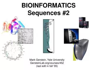
BIOINFORMATICSSequences Mark Gerstein, Yale University gersteinlab.org/courses/452 (last edit in spring ‘10, final edit)
Basic Alignment via Dynamic Programming Suboptimal Alignment Gap Penalties Similarity (PAM) Matrices Multiple Alignment Profiles, Motifs, HMMs Local Alignment Probabilistic Scoring Schemes Rapid Similarity Search: Fasta Rapid Similarity Search: Blast Practical Suggestions on Sequence Searching Transmembrane helix predictions Secondary Structure Prediction: Basic GOR Secondary Structure Prediction: Other Methods Assessing Secondary Structure Prediction Features of Genomic DNA sequences Sequence Topics (Contents)
Raw Data ???T C A T G C A T T G 2 matches, 0 gaps T C A T G | |C A T T G 3 matches (2 end gaps) T C A T G . | | | . C A T T G 4 matches, 1 insertion T C A - T G | | | | . C A T T G 4 matches, 1 insertion T C A T - G | | | | . C A T T G Core Aligning Text Strings
Dynamic Programming • What to do for Bigger String? SSDSEREEHVKRFRQALDDTGMKVPMATTNLFTHPVFKDGGFTANDRDVRRYALRKTIRNIDLAVELGAETYVAWGGREGAESGGAKDVRDALDRMKEAFDLLGEYVTSQGYDIRFAIEP KPNEPRGDILLPTVGHALAFIERLERPELYGVNPEVGHEQMAGLNFPHGIAQALWAGKLFHIDLNGQNGIKYDQDLRFGAGDLRAAFWLVDLLESAGYSGPRHFDFKPPRTEDFDGVWAS • Needleman-Wunsch (1970) provided first automatic method • Dynamic Programming to Find Global Alignment • Their Test Data (J->Y) • ABCNYRQCLCRPMAYCYNRCKCRBP
Step 1 -- Make a Dot Plot (Similarity Matrix) Core Put 1's where characters are identical.
A More Interesting Dot Matrix (adapted from R Altman)
Core Step 2 -- Start Computing the Sum Matrix new_value_cell(R,C) <= cell(R,C) { Old value, either 1 or 0 } + Max[ cell (R+1, C+1), { Diagonally Down, no gaps } cells(R+1, C+2 to C_max),{ Down a row, making col. gap } cells(R+2 to R_max, C+1) { Down a col., making row gap } ]
Core Step 2 -- Start Computing the Sum Matrix new_value_cell(R,C) <= cell(R,C) { Old value, either 1 or 0 } + Max[ cell (R+1, C+1), { Diagonally Down, no gaps } cells(R+1, C+2 to C_max),{ Down a row, making col. gap } cells(R+2 to R_max, C+1) { Down a col., making row gap } ]
Core Step 3 -- Keep Going
Core Step 4 -- Sum Matrix All Done Alignment Score is 8 matches.
Core Step 5 -- Traceback Find Best Score (8) and Trace BackA B C N Y - R Q C L C R - P MA Y C - Y N R - C K C R B P Hansel & Gretel
Core Step 6 -- Alternate Tracebacks A B C - N Y R Q C L C R - P MA Y C Y N - R - C K C R B P Also, Suboptimal Aligments
Suboptimal Alignments ; ; Random DNA sequence generated using the seed : -453862491 ; ; 500 nucleotides ; ; A:C:G:T = 1 : 1 : 1 : 1 ; RAN -453862491 AAATGCCAAA TCATACGAAC AGCCGACGAC GGGAGCAACC CAAGTCGCAG TTCGCTTGAG CTAGCGCGCT CCCACCGGGA TATACACTAA TCATTACAGC AGGTCTCCTG GGCGTACAGA CTAGCTGAAC GCGCTGCGCC AATTCCAACT TCGGTATGAA GGATCGCCTG CGGTTATCGC TGACTTGAGT AACCAGATCG CTAAGGTTAC GCTGGGGCAA TGATGGATGT TAACCCCTTA CAGTCTCGGG AGGGACCTTA AGTCGTAATA GATGGCAGCA TTAATACCTT CGCCGTTAAT ATACCTTTAA TCCGTTCTTG TCAATGCCGT AGCTGCAGTG AGCCTTCTGT CACGGGCATA CCGCGGGGTA GCTGCAGCAA CCGTAGGCTG AGCATCAAGA AGACAAACAC TCCTCGCCTA CCCCGGACAT CATATGACCA GGCAGTCTAG GCGCCGTTAG AGTAAGGAGA CCGGGGGGCC GTGATGATAG ATGGCGTGTT 1 ; ; Random DNA sequence generated using the seed : 1573438385 ; ; 500 nucleotides ; ; A:C:G:T = 1 : 1 : 1 : 1 ; RAN 1573438385 CCCTCCATCG CCAGTTCCTG AAGACATCTC CGTGACGTGA ACTCTCTCCA GGCATATTAA TCGAAGATCC CCTGTCGTGA CGCGGATTAC GAGGGGATGG TGCTAATCAC ATTGCGAACA TGTTTCGGTC CAGACTCCAC CTATGGCATC TTCCGCTATA GGGCACGTAA CTTTCTTCGT GTGGCGGCGC GGCAACTAAA GACGAAAGGA CCACAACGTG AATAGCCCGT GTCGTGAGGT AAGGGTCCCG GTGCAAGAGT AGAGGAAGTA CGGGAGTACG TACGGGGCAT GACGCGGGCT GGAATTTCAC ATCGCAGAAC TTATAGGCAG CCGTGTGCCT GAGGCCGCTA GAACCTTCAA CGCTAACTAG TGATAACTAC CGTGTGAAAG ACCTGGCCCG TTTTGTCCCT GAGACTAATC GCTAGTTAGG CCCCATTTGT AGCACTCTGG CGCAGACCTC GCAGAGGGAC CGGCCTGACT TTTTCCGGCT TCCTCTGAGG 1 Parameters: match weight = 10, transition weight = 1, transversion weight = -3 Gap opening penalty = 50 Gap continuation penalty = 1 Run as a local alignment (Smith-Waterman) (courtesy of Michael Zucker)
Suboptimal Alignments II (courtesy of Michael Zucker)
Core Gap Penalties The score at a position can also factor in a penalty for introducing gaps (i. e., not going from i, j to i- 1, j- 1). Gap penalties are often of linear form: GAP = a + bN GAP is the gap penalty a = cost of opening a gap b = cost of extending the gap by one (affine) N = length of the gap (Here assume b=0, a=1/2, so GAP = 1/2 regardless of length.) ATGCAAAAT ATG-AAAAT .5 ATG--AAAT .5 + (1)b [b=.1] ATG---AAT .5 + (2)(.1) =.7
Step 2 -- Computing the Sum Matrix with Gaps Core new_value_cell(R,C) <= cell(R,C) { Old value, either 1 or 0 } + Max[ cell (R+1, C+1), { Diagonally Down, no gaps } cells(R+1, C+2 to C_max) - GAP ,{ Down a row, making col. gap } cells(R+2 to R_max, C+1) - GAP { Down a col., making row gap } ] GAP =1/2 1.5
C R B P C R P M - C R P M C R - P M All Steps in Aligning a 4-mer Bottom right hand corner of previous matrices
ACSQRP--LRV-SH RSENCVA-SNKPQLVKLMTH VKDFCV ACSQRP--LRV-SH -R SENCVA-SNKPQLVKLMTH VK DFCV Key Idea in Dynamic Programming • The best alignment that ends at a given pair of positions (i and j) in the 2 sequences is the score of the best alignment previous to this position PLUS the score for aligning those two positions. • An Example Below • Aligning R to K does not affect alignment of previous N-terminal residues. Once this is done it is fixed. Then go on to align D to E. • How could this be violated? Aligning R to K changes best alignment in box.
Core Similarity (Substitution) Matrix A R N D C Q E G H I L K M F P S T W Y V A 4 -1 -2 -2 0 -1 -1 0 -2 -1 -1 -1 -1 -2 -1 1 0 -3 -2 0 R -1 5 0 -2 -3 1 0 -2 0 -3 -2 2 -1 -3 -2 -1 -1 -3 -2 -3 N -2 0 6 1 -3 0 0 0 1 -3 -3 0 -2 -3 -2 1 0 -4 -2 -3 D -2 -2 1 6 -3 0 2 -1 -1 -3 -4 -1 -3 -3 -1 0 -1 -4 -3 -3 C 0 -3 -3 -3 8 -3 -4 -3 -3 -1 -1 -3 -1 -2 -3 -1 -1 -2 -2 -1 Q -1 1 0 0 -3 5 2 -2 0 -3 -2 1 0 -3 -1 0 -1 -2 -1 -2 E -1 0 0 2 -4 2 5 -2 0 -3 -3 1 -2 -3 -1 0 -1 -3 -2 -2 G 0 -2 0 -1 -3 -2 -2 6 -2 -4 -4 -2 -3 -3 -2 0 -2 -2 -3 -3 H -2 0 1 -1 -3 0 0 -2 7 -3 -3 -1 -2 -1 -2 -1 -2 -2 2 -3 I -1 -3 -3 -3 -1 -3 -3 -4 -3 4 2 -3 1 0 -3 -2 -1 -3 -1 3 L -1 -2 -3 -4 -1 -2 -3 -4 -3 2 4 -2 2 0 -3 -2 -1 -2 -1 1 K -1 2 0 -1 -3 1 1 -2 -1 -3 -2 5 -1 -3 -1 0 -1 -3 -2 -2 M -1 -1 -2 -3 -1 0 -2 -3 -2 1 2 -1 5 0 -2 -1 -1 -1 -1 1 F -2 -3 -3 -3 -2 -3 -3 -3 -1 0 0 -3 0 6 -4 -2 -2 1 3 -1 P -1 -2 -2 -1 -3 -1 -1 -2 -2 -3 -3 -1 -2 -4 6 -1 -1 -4 -3 -2 S 1 -1 1 0 -1 0 0 0 -1 -2 -2 0 -1 -2 -1 4 1 -3 -2 -2 T 0 -1 0 -1 -1 -1 -1 -2 -2 -1 -1 -1 -1 -2 -1 1 5 -2 -2 0 W -3 -3 -4 -4 -2 -2 -3 -2 -2 -3 -2 -3 -1 1 -4 -3 -2 10 2 -3 Y -2 -2 -2 -3 -2 -1 -2 -3 2 -1 -1 -2 -1 3 -3 -2 -2 2 6 -1 V 0 -3 -3 -3 -1 -2 -2 -3 -3 3 1 -2 1 -1 -2 -2 0 -3 -1 4 • Identity Matrix • Match L with L => 1Match L with D => 0Match L with V => 0?? • S(aa-1,aa-2) • Match L with L => 1Match L with D => 0Match L with V => .5 • Number of Common Ones • PAM • Blossum • Gonnet
+ —> More likely than random 0 —> At random base rate - —> Less likely than random Where do matrices come from? 1 Manually align protein structures(or, more risky, sequences) 2 Look at frequency of a.a. substitutionsat structurally constant sites. -- i.e. pair i-j exchanges 3 Compute log-odds S(aa-1,aa-2) = log2 ( freq(O) / freq(E) ) O = observed exchanges, E = expected exchanges • odds = freq(observed) / freq(expected) • Sij = log odds • freq(expected) = f(i)*f(j) = is the chance of getting amino acid i in a column and then having it change to j • e.g. A-R pair observed only a tenth as often as expected 90% AAVLL… AAVQI… AVVQL… ASVLL… 45% Core
Relationship of type of substitution to closeness in identity of the sequences in the training alignment
Different Matrices are Appropriate at Different Evolutionary Distances Core Different gold std. sets of seq at diff ev. dist. --> matrices Ev. Equiv. seq. (ortholog) [hb and mb] (Adapted from D Brutlag, Stanford)
PAM-250 (distant) Change in Matrix with Ev. Dist. Chemistry (far) v genetic code (near) PAM-78 (Adapted from D Brutlag, Stanford)
Some concepts challenged: Are the evolutionary rates uniform over the whole of the protein sequence? (No.) The BLOSUM matrices: Henikoff & Henikoff (Henikoff, S. & Henikoff J.G. (1992) PNAS89:10915-10919) . This leads to a series of matrices, analogous to the PAM series of matrices. BLOSUM80: derived at the 80% identity level. The BLOSUM Matrices BLOSUM62 is the BLAST default Blossum40 is for far things
Modifications for Local Alignment Core 1 The scoring system uses negative scores for mismatches 2 The minimum score for at a matrix element is zero 3 Find the best score anywhere in the matrix (not just last column or row) • These three changes cause the algorithm to seek high scoring subsequences, which are not penalized for their global effects (mod. 1), which don’t include areas of poor match (mod. 2), and which can occur anywhere (mod. 3) (Adapted from R Altman)
Global (NW) vs Local (SW)Alignments mismatch T T G A C A C C... | | - | | | | - T T T A C A C A... 1 2 1 2 3 4 5 4 0 0 4 4 4 4 4 8 TTGACACCCTCCCAATTGTA... |||||| | .....ACCCCAGGCTTTACACAT 123444444456667 Match Score = +1Gap-Opening=-1.2, Gap-Extension=-.03for local alignment Mismatch = -0.6 Adapted from D J States & M S Boguski, "Similarity and Homology," Chapter 3 from Gribskov, M. and Devereux, J. (1992). Sequence Analysis Primer. New York, Oxford University Press. (Page 133)
Shows Numbers Match Score = 1, Gap-Opening=-1.2, Gap-Extension=-.03, for local alignment Mismatch = -0.6 Local Global Adapted from D J States & M S Boguski, "Similarity and Homology," Chapter 3 from Gribskov, M. and Devereux, J. (1992). Sequence Analysis Primer. New York, Oxford University Press. (Page 133)
Local vs. Global Alignment Core • GLOBAL = best alignment of entirety of both sequences • For optimum global alignment, we want best score in the final row or final column • Are these sequences generally the same? • Needleman Wunsch • find alignment in which total score is highest, perhaps at expense of areas of great local similarity • LOCAL = best alignment of segments, without regard to rest of sequence • For optimum local alignment, we want best score anywhere in matrix (will discuss) • Do these two sequences contain high scoring subsequences • Smith Waterman • find alignment in which the highest scoring subsequences are identified, at the expense of the overall score (Adapted from R Altman)
The Score S = Total Score S(i,j) = similarity matrix score for aligning i and j Sum is carried out over all aligned i and j n = number of gaps (assuming no gap ext. penalty) G = gap penalty Core Simplest score (for identity matrix) is S = # matches What does a Score of 10 mean? What is the Right Cutoff?
Score in Context of Other Scores • How does Score Rank Relative to all the Other Possible Scores • P-value • Percentile Test Score Rank • All-vs-All comparison of the Database (100K x 100K) • Graph Distribution of Scores • ~1010 scores much smaller number of true positives • N dependence Core
P-value in Sequence Matching • P(s > S) = .01 • P-value of .01 occurs at score threshold S (392 below) where score s from random comparison is greater than this threshold 1% of the time • Likewise for P=.001 and so on. Core
P-values Core 1 • Significance Statistics • For sequences, originally used in Blast (Karlin-Altschul). Then in FASTA, &c. • Extrapolated Percentile Rank: How does a Score Rank Relative to all Other Scores? • Our Strategy: Fit to Observed Distribution 1) All-vs-All comparison 2) Graph Distribution of Scores in 2D (N dependence); 1K x 1K families -> ~1M scores; ~2K included TPs 3) Fit a function r(S) to TN distribution (TNs from scop); Integrating r gives P(s>S), the CDF, chance of getting a score better than threshold S randomly 4)Use same formalism for sequence & structure 2 [ e.g. P(score s>392) = 1% chance] 3
Reasonable as Dyn. Prog. maximizes over pseudo-random variables EVD is Max(indep. random variables); Normal is Sum(indep. random variables) EVD Fits Observed r(z) = exp(-z2) ln r(z) = -z2 Extreme Value Distribution (EVD, long-tailed) fits the observed distributions best. The corresponding formula for the P-value: Core
Extreme Value vs. Gaussian • X = set of random numbers Each set indexed by j • j=1: 1,4,9,1,3,1 • j=2: 2,7,3,11,22,1,22 • Gaussian S(j) = j Xi[central limit] • EVD S(j) = max(Xi) Freq. S(j)
Objective is to Find Distant Homologues • Score (Significance) Threshold • Maximize Coverage with an Acceptable Error Rate • TP, TN, FP, FN • TP and TN are good! • We get *P and *N from our program • We get T* and F* from a gold-standard • Max(TP,TN) vs (FP,FN) (graphic adapted from M Levitt)
100% 100% Core Coverage v Error Rate (ROC Graph) Coverage (roughly, fraction of sequences that one confidently “says something” about) Thresh=10 Thresh=20 [sensitivity=tp/p=tp/(tp+fn)] Thresh=30 Different score thresholds Error rate (fraction of the “statements” that are false positives) Two “methods” (red is more effective) [Specificity = tn/n =tn/(tn+fp)] error rate = 1-specificity = fp/n
Significance Dependson Database Size • The Significance of Similarity Scores Decreases with Database Growth • The score between any pair of sequence pair is constant • The number of database entries grows exponentially • The number of nonhomologous entries >> homologous entries • Greater sensitivity is required to detect homologiesGreater s • Score of 100 might rank as best in database of 1000 but only in top-100 of database of 1000000 DB-1 DB-2
Low-Complexity Regions • Low Complexity Regions • Different Statistics for matching AAATTTAAATTTAAATTTAAATTTAAATTTthanACSQRPLRVSHRSENCVASNKPQLVKLMTHVKDFCV • Automatic Programs Screen These Out (SEG) • Identify through computation of sequence entropy in a window of a given size H = f(a) log2 f(a) • Also, Compositional Bias • Matching A-rich query to A-rich DB vs. A-poor DB Core LLLLLLLLLLLLL
N M M’ N’ Computational Complexity Core • Basic NW Algorithm is O(n2) (in speed) • M x N squares to fill • At each square need to look back (M’+N’) “black” squares to find max in block • M x N x (M’+N’) -> O(n3) • However, max values in block can be cached, so algorithm is really only O(n2) • O(n2) in memory too! • Improvements can (effectively) reduce sequence comparison to O(n) in both
FASTA Core • Hash table of short words in the query sequence • Go through DB and look for matches in the query hash (linear in size of DB) • perl: $where{“ACT”} = 1,45,67,23.... • K-tuple determines word size (k-tup 1 is single aa) • by Bill Pearson VLICT = _ VLICTAVLMVLICTAAAVLICTMSDFFD
Join together query lookups into diagonals and then a full alignment (Adapted from D Brutlag)
Basic Blast • Altschul, S., Gish, W., Miller, W., Myers, E. W. & Lipman, D. J. (1990). Basic local alignment search tool. J. Mol. Biol.215, 403-410 • Indexes query • BLAT - indexes DB • Starts with all overlapping words from query • Calculates “neighborhood” of each word using PAM matrix and probability threshold matrix and probability threshold • Looks up all words and neighbors from query in database index • Extends High Scoring Pairs (HSPs) left and right to maximal length • Finds Maximal Segment Pairs (MSPs) between query and database • Blast 1 does not permit gaps in alignments Core
Blast: Extension of Hash Hits Core • Extend hash hits into High Scoring Segment Pairs (HSPs) • Stop extension when total score doesn’t increase • Extension is O(N). This takes most of the time in Blast Query DB
Blasting against the DB • In simplest Blast algorithm, find best scoring segment in each DB sequence • Statistics of these scores determine significance Number of hash hits is proportional to O(N*M*D), where N is the query size, M is the average DB seq. size, and D is the size of the DB
Blast2: Gapped Blast Core
Blast2: Gapped Blast • Gapped Extension on Diagonals with two Hash Hits • Statistics of Gapped Alignments follows EVD empirically Core
Examine results with exp. between 0.05 and 10 Reevaluate results of borderline significance using limited query Beware of hits on long sequences Limit query length to 1,000 bases Segment query if more than 1,000 bases Search both strands Protein search is more sensitive, Translate ORFs BLAST for infinite gap penalty Smith-Waterman for cDNA/genome comparisons cDNA =>Zero gap-Transition matrices Consider transition matrices Ensure that expected value of score is negative Practical Issues on DNA Searching (graphic and some text adapted from D Brutlag)
Choose between local or global search algorithms Use most sensitive search algorithm available Original BLAST for no gaps Smith-Waterman for most sensitivity FASTA with k-tuple 1 is a good compromise Gapped BLAST for well delimited regions PSI-BLAST for families(differential performance on large and small families) Initially BLOSUM62 and default gap penalties If no significant results, use BLOSUM30 and lower gap penalties FASTA cutoff of .01 Blast cutoff of .0001 Examine results between exp. 0.05 and 10 for biological significance Ensure expected score is negative Beware of hits on long sequences or hits with unusual aa composition Reevaluate results of borderline significance using limited query region Segment long queries ³ 300 amino acids Segment around known motifs General Protein Search Principles (some text adapted from D Brutlag)