
Fast Hough Transform Method
E N D
Presentation Transcript
Fast Hough Transform Method Cvetan Cheshkov ALICE offline week
Contents • Introduction • Fast Hough Transform method • Demo • Results on timing, efficiency and resolution • Concluding remarks and future plans ALICE offline week
HLT (high multiplicity case) Hough Transform Local Peak finder TPC digits Find, deconvolute and associate clusters Track fit • Hough Transform takes 1000-2300s in linear mode (dn/dy3500; PIII 800MHz) ALICE offline week
Hough Transform (HT) • Each TPC digit is transformed into a curve in the Hough parameter space corresponding to all possible tracks to which the digit could be associated: (x,y)(k=1/R,) k – track curvature; - track emission angle • The Hough approach: • Assumes that the tracks are coming from (or close to) the primary vertex • Neglects any energy losses and multiply scattering in the detector volume ALICE offline week
HLT implementation of HT • TPC data input is splitted in sectors, r/o patchesand slices (50-100) • Hough transform is performed on each of these slices separately (in parallel) • The HT parameter space is binned and stored in histograms • The histograms are summed over the patches • Local peaks are identified by a peak finder and transmitted as track seeds to the cluster finder ALICE offline week
Improving HT • Originally HT was done filling the digits charge Large amount of fakes in a high occupancy case Sophisticated peak finder • Studying the HT performance it turned out that the performance can be improved by counting: digits charge #digits #clusters (TPC rows) ALICE offline week
“Counting Rows & Gaps” HT • Naturally the studies lead to the idea to count consecutive TPC rows • Idea: Good track candidate must have not only some amount of digit’s charge, digits or rows along its trajectory, but also must occupy consecutive TPC rows • Now the algorithm counts as #gaps between occupied rows • Weight used to fill HT space: • #rows/#gaps • #rows (#gaps<N) ALICE offline week
Example Corresponding HT space Slice of 1 TPC sector • Central HIJING dn/dy=3500, 0.2T ALICE offline week
New Peak Finder (PF) • The improvement in the HT quality simpler PF • The new PF looks for neighbor bins with the same weight • Track parameters are extracted by averaging the peak edge points both in and 1/R (track curvature) directions track is guided by the cluster borders ALICE offline week
Comparison Standard HT New HT • New Hough seeds much more clear • It seems that now the cluster fitter is • the limiting factor (it is also the slowest part) ALICE offline week
Fast Hough Transform • Assuming ordered TPC digits (in time bins, pads, padrows) new algorithm offers big space for speeding up • HT is monotonic along the padrows do it only for the first and last (in paw index direction) digits which belong to a cluster and fill a the corresponding ribbon in the HT space • Stopping rules using already accumulated #gaps ALICE offline week
Fast Hough Transform • By introducing the new HT and substituting sin and cos by LUTs a factor of 10 in the speed 2300s 230s • Which are the sources: • LUTs - factor of 2 • HT algorithm – factor of 5 • Additional factor of 2 • Code improvement • #gaps stopping rule • Filter on the data (consistent with HT algorithm) ALICE offline week
Demo! • Demo with central HIJING event (dn/dy=3500) on one of the GDCs (oplapro machines) used in the Computing DC • The event is stored as DATE formatted file and is processed by a stand-alone exe (see Thomas’ talk) • Oplapro – Itanium II; 1.5GHz; 4Mb L3 cache ALICE offline week
Timings • HT space size: • (75 in )x(140 in 1/R)x(100 in ) • Time consumption is: • strictly proportional to the HT space size • roughly proportional to the event multiplicity ALICE offline week
Performance • Try to run Hough stand-alone (without a consecutive cluster fitter and etc) • The method requires new definitions in order to determine the performance: • No clusters associated assign only 1 MC label to each track • High occupancy (and therefore overlapping clusters) in general does not affect the track parameters, but cause appearance of “ghosts” fakes tracks ghost tracks • If more than 1 track with the same MC label, take randomly one as good and second as ghost • Good tracks – primaries from offline comparison ALICE offline week
Performance /Efficiencies/ Parameterized HIJING dn/dy=8000 B=0.2T B=0.4T B=0.5T ALICE offline week
Performance /Efficiencies/ dn/dy=2000 dn/dy=4000 B=0.2T B=0.4T B=0.4T ALICE offline week
Performance /Efficiency/ • Summary: • The efficiency is almost unaffected by the event multiplicity!! • About ½ of the ghosts are coming from the high occupancy ALICE offline week
Performance /Resolution/ Parameterized HIJING dn/dy=4000, 0.4T Pt/Pt(%)=0.7+2.7xPt =6.3x10-3 =7.2mrad ALICE offline week
Performance /Resolution/ • Summary: • The relative Pt resolution rises linearly with Pt consistent with the expectations from HT binning! • It is almost proportional to 1/B • The resolution on eta,psi and Pt (high Pt tracks) increase by <10% when dn/dy goes from 2000 to 8000 (the effect is due mostly to ghosts) • At low Pt one can see clearly the effect of ghosts ALICE offline week
Known problems • The Peak Finder has certain problems with the cut on the peaks size • The main source of inefficiencies • We need cut which depends on the position inside Hough space • Special treatment of tracks crossing 2 sectors • They give significant contribution to the #ghosts • Need in a proper global (between eta slices and sectors) track merger! ALICE offline week
Concluding remarks • The new Hough method shows reasonable performance and is much much faster! • Needs some further optimization and evaluation • The answer about its applicability can be given only by trying some real physics trigger algorithms (hopefully using PDC’04 data) ALICE offline week
Concluding remarks • Impact on physics cases: • Jet finder • The efficiency for Pt above 2-2.5 GeV is high • The ghosts almost disappear at 2.5 GeV • The eta and psi resolutions are pretty good for any cone jet-finder sizes (0.1,0.2,…) • The Pt resolution for high Pt tracks does not explode • Open charm track filter • The efficiency between 0.5 and 1 GeV looks reasonable • The ghosts in principle do not hurt too much because they are close to the good tracks ALICE offline week
Future plans • Next week everything to CVS • Work on Peak Finder and investigation of inefficiencies and ghosts • Preparation of physics trigger algorithms and their evaluation • As soon as Computing DC is restarted try the whole machinery in online mode • Closer integration with AliRoot ALICE offline week