
Viscoelastic Response in Soft Matter: From Lennard-Jones Potentials to Glass Transition
E N D
Presentation Transcript
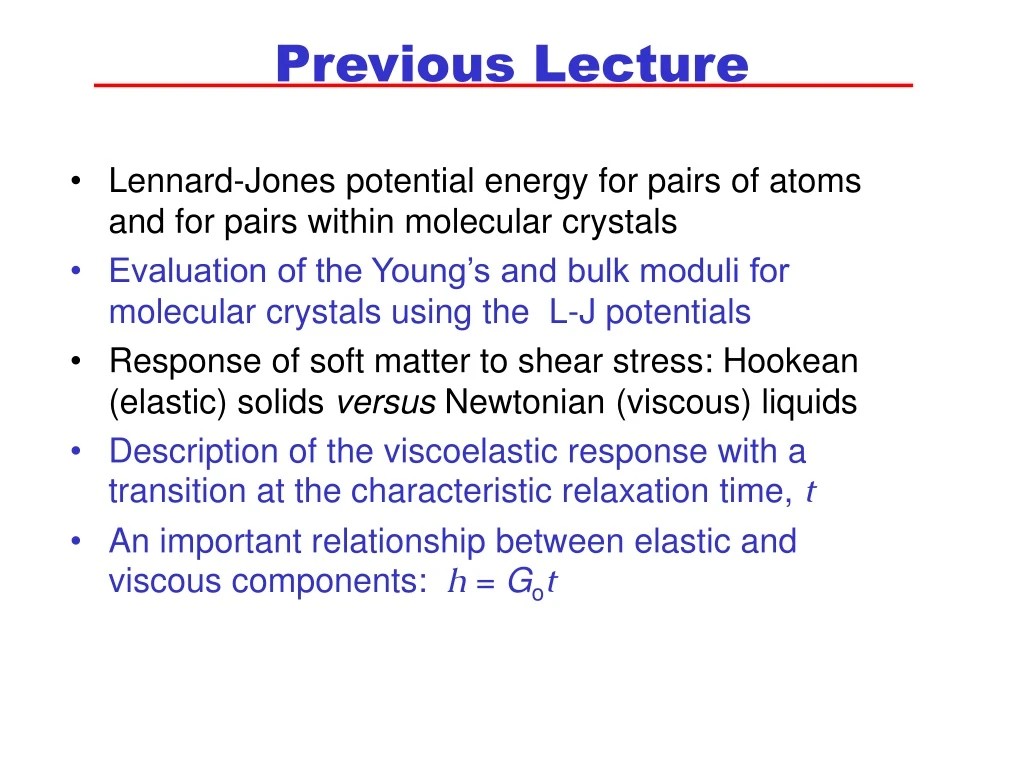
Previous Lecture • Lennard-Jones potential energy for pairs of atoms and for pairs within molecular crystals • Evaluation of the Young’s and bulk moduli for molecular crystals using the L-J potentials • Response of soft matter to shear stress: Hookean (elastic) solids versus Newtonian (viscous) liquids • Description of the viscoelastic response with a transition at the characteristic relaxation time, t • An important relationship between elastic and viscous components: h = Got
3SMS Lecture 4 Time Scales, the Glass Transition and Glasses, and Liquid Crystals 6 February, 2007 See Jones’ Soft Condensed Matter, Chapt. 2 and 7
Slope: tis the relaxation time t Response of Soft Matter to a Constant Shear Stress: Viscoelasticity t We see that 1/Go (1/h)t An alternative expression for viscosity is thus h Got
Relaxation and a Simple Model of Viscosity F • When a liquid is subjected to a shear stress, immediately the molecules’ positions are shifted but the same “neighbours” are kept. • Thereafter, the constituent molecules re-arrange to relax the stress, and the liquid begins to flow. • A simple model of liquids imagines that relaxation takes place by a hopping mechanism, in which molecules escape the “cage” formed by its neighbours. • Molecules in a liquid vibrate with a frequency, n,comparable to the phonon frequency in a solid of the same substance. • Thus n can be considered a frequency of attempts to escape a cage. • But what is the probability that the molecule will escape the cage?
Intermediate state: some molecular spacings are greater e Potential Energy 0 Molecular configuration Need to consider the probability of being in a higher state with an energy of e.
Molecular Relaxation Time • eis the energy of the higher state and can be considered an energy barrier per molecule. • Typically, e 0.4 Lv/NA, where Lv is the heat of vapourisation per mole and NA is the Avogadro number. • At statistical argument tells us that the probability P of being in the high energy state is given by the Boltzmann distribution: P ~ exp(-e /kT) • T is the temperature of the reservoir. As T 0, then P0, whereas when T, then P1 (100% success) • Eyring proposed that the frequency of successful escapes, f, is then the product of the frequency of attempts (n) and the probability of success (P): The time required for a molecule to escape its cage defines a molecular relaxation time,t, which is comparable in magnitude to the macroscopic relaxation time. And so, t = 1/f.
Arrhenius Behaviour of Viscosity • In liquids, t is very short, varying between 10-12 and 10-10 s. Hence, as commonly observed, stresses in liquids are relaxed nearly instantaneously. • In melted polymers, t is on the order of several ms or s. • From our discussion of viscoelasticity, we know that h Got. Hence an expression for h can be found from the Eyring relationship: Alternatively, an expression based on the molar activation energy E can be written: This is referred to as an Arrhenius relationship.
where B and To are empirical constants. (By convention, the units of temp. here are usually °C!) Non-Arrhenius Temperature Dependence • Liquids with a viscosity that shows an Arrhenius dependence on temperature are called “strong liquids”. An example is melted silica. • “Fragile liquids” show a non-Arrhenius behaviour that requires a different description. • An example of a fragile liquid is a melted polymer, which is described by the Vogel-Fulcher relationship: We see that h diverges to , as the liquid is cooled towards To. It solidifies as temperature is decreased. In the high-temperature limit, h approaches ho - a lower limit.
Temperature-Dependence of Viscosity Arrhenius V-F P = Poise
Configurational Re-Arrangements • As a liquid is cooled, stress relaxation takes longer, and it takes longer for the molecules to change their configuration, as described by the configurational relaxation time, tconfig. • From the Vogel-Fulcher equation, we see that: We see that the relaxations become exceedingly slow as T decreases towards To.
Debonding of an Adhesive Experimental Time Scales • To distinguish a liquid from a solid, flow (or other liquid-like behaviour) must be observed on an experimental time scale, texp. A substance will appear to be a solid on short time scales but a liquid on long time scales! • For example, if a sample is being cooled at a rate of 1 K per min., then texp is ~1 min. at each temperature increment. Flow is observed on long time scales, texp At higher temperatures, texp > tconfig, and flow is observed on the time scale of the measurement.
Oscillatory Stress Apply a shear stress (or strain) at an angular frequency of = 1/texp ss t 1/
Are Stained-Glass Windows Liquid? Some medieval church windows are thicker at their bottom. Is there flow over a time scale of texp100 years? Window in the Duomo of Siena
The Glass Transition • At higher temperatures, texp > tconfig, and so flow is observed on the time scale of the measurement. • As T is lowered, tconfig increases. • When T is decreased to a certain value, known as the glass transition temperature, Tg, then tconfig ~ texp. • Below Tg, molecules do not change their configuration sufficiently fast to be observed during texp. That is, texp < tconfig. The substance appears to be solid-like, with no observable flow. • At T = Tg, h is typically 1013 Pas. Compare this to h = 10 -3 Pas for water at room temperature.
1/texp 1/Tg Competing Time Scales =1/tvib Log(1/t) tconfig < texp f = 1/tconfig Melt (liquid) tconfig > texp glass Reciprocal Temperature (K-1)
Effect of Cooling Rate on Tg • Tg is not a constant for a substance. • When the cooling rate is slower,texp is longer. • For instance, reducing the rate from 1 K min-1 to 0.1 K min-1, increases texp from 1 min. to 10 min. at each increment in K. • With a slower cooling rate, a lower T can be reached before tconfig texp. • The result is a lower observed Tg. • Various experimental techniques have different associated texp values. Hence, a value of Tg depends on the technique used to measure it.
Thermodynamics of Phase Transitions • How can we classify the glass transition? • At equilibrium, the stable phase will have the lowest Gibbs free energy. • During a transition from solid to liquid, we see that will be discontinuous:
Classification of Phase Transitions • A phase transition is classified as “first-order” if the first derivative of the Gibbs’ Free Energy, G, with respect to any state variable is discontinuous. • An example - from the previous page - is the melting transition. • In the same way, in a “second-order” phase transition, the second derivative of the Gibbs’ Free Energy G is discontinuous. • Examples include order-disorder phase transitions in metals and superconducting/non-SC transitions.
Thermodynamics of First-Order Transitions • Gibbs’ Free Energy, G: G = H-ST so that dG = dH - TdS - SdT • Enthalpy, H = U+PV so that dH = dU + PdV + VdP • Substituting in for dH, we see: dG = dU + PdV + VdP - TdS - SdT • The central equation of thermodynamics tells us: dU = SdT - PdV • Substituting for dU, we find: dG = SdT - PdV + PdV + VdP - TdS - SdT S = entropy U = internal energy Finally, dG = VdP-TdS
V There is a heat of melting, and thus H is discontinuous at Tm. liquid (Or H) crystalline solid Tm T Thermodynamics of First-Order Transitions • dG = VdP - TdS • In a first order transition, we see that V and S must be discontinuous: Viscosity is also discontinuous at Tm.
Glass Tg Tm Thermodynamics of Glass Transitions V Liquid Crystalline solid T
Thermodynamics of Glass Transitions Faster-cooled glass Glass Tg Tm Tfcg Tg is higher when there is a faster cooling rate. We see that the density of a glass is a function of its “thermal history”. V Liquid Crystalline solid T
And V = (dG/dP)S. So, Expansivity is likewise discontinuous in a second-order phase transition. Is the Glass Transition Second-Order? • Note that dS is found from -(dG/dT)P. Then we see that the heat capacity, Cp, can be given as: • Thus in a second-order transition, CP will be discontinuous. • Recall that volume expansivity, b, is defined as:
Experimental Results for Poly(Vinyl Acetate) Data from Kovacs
Melt Glass Tg Determining the Glass Transition Temperature in Polymer Thin Films Poly(styrene) ho ~ 100 nm ~ Thickness Keddie et al., Europhys. Lett. 27 (1994) 59-64
Glass Transition of Poly(vinyl chloride) Sample is heated at a constant rate. Calorimeter measures how much heat is required. Heat flow ~ heat capacity T Data from H. Utschick, TA Instruments
Structure of Glasses • There is no discontinuity in volume at the glass transition and nor is there a discontinuity in the structure. • In a crystal, there is long-range order of atoms. They are found at predictable distances. • But at T>0, the atoms vibrate about an average position, and so the position is described by a distribution of probable interatomic distances, n(r).
Atomic Distribution in Crystals 12 nearest neighbours And 4th nearest! FCC unit cell (which is repeated in all three directions)
Comparison of Glassy and Crystalline Structures 2-D Structures Local order is identical in both structures Crystalline Glassy (amorphous) Going from glassy to crystalline, there is a discontinuous decrease in volume.
Structure of Glasses and Liquids • The structure of glasses and liquids can be described by a radial distribution function: g(r), where r is the distance from the centre of a reference atom/molecule. • The density in a shell of radius r will have r atoms per volume. • For the entire substance, let there be ro atoms per unit volume. Then g(r) = r(r)/ro. • At short r, there is some predictability of position because short-range forces are operative. • At long r, r(r) approaches ro and g(r) 1.
R.D.F. for Liquid Argon Experimentally, vary a wave vector: Scattering occurs when: (where d is the spacing). Can very either q or l in experiments
R.D.F. for Liquid Sodium Compared to the BCC Crystal 4pr2r(r) 3 BCC cells Each Na has 8 nearest neighbours. r (Å)
Entropy of Glasses • Entropy,S, can be determined experimentally from integrating plots of CP/T versus T (since Cp = T(dS/dT)P) • The disorder (and S) in a glass is similar to that in the melt. Compare to crystallisation in which S jumps down at Tm. • Since the glass transition is not first-order, S is not discontinuous through the transition. • S for a glass depends on the cooling rate. • As the cooling rate becomes slower, S becomes lower. • At a temperature called the Kauzmann temperature, TK, we expect that Sglass = Scrystal. • The structure of a glass is similar to the liquid’s, but there is greater disorder in the glass compared to the crystal of the same substance.
Kauzmann Paradox Melt (Liquid) Glass Crystal
Kauzmann Paradox • Sglass cannot be less than Scrystal. • Yet by extrapolation, we can predict that at sufficiently slow cooling rate, Sglass will be less than Scrystal. This prediction is a paradox! • Paradox is resolved by saying that TK defines a lower limit to Tg as given by the V-F equation. • Experimentally, it is usually found that TK To (V-F constant). Typically, Tg - To = 50 K. • This is consistent with the prediction that at T = To, tconfig will go to . • Tg equals TK (and To) when texp is approaching , which would be obtained via an exceedingly slow cooling rate.
Liquid Crystals Rod-like (= calamitic) molecules Molecules can also be plate-like (= discotic)
Density Temp. LC Phases N = director Isotropic The phases ofthermotropicLCs depend on the temperature. Nematic Attractive van der Waals’ forces are balanced by forces from thermal motion. Smectic
Density Order in LC Phases N = director OrientationalPositional None weak 1-D 1-D None High High High Isotropic Nematic Smectic
n Director N N LC Orientation Distribution function, f(q) Higher order Lower order p 0
Order Parameter for a Nematic-Isotropic LC Transition The molecular ordering in a LC can be described by a so-called order parameter, S: S 1 Nematic With the greatest ordering, q = 0° and S = 1. Isotropic Discontinuity at Tc: Therefore, a first-order transition 0 The order parameter is determined by the minimum in the free energy, F. Disordering increases S and decreases F, BUT intermolecular energies and F are decreased with ordering.
Scattering Experiments q l d = molecular spacing
Polarised Light Microscopy of LC Phases Why do LCs show birefringence? (That is, their refractive index varies with direction in the substance.) Nematic LC
In the isotropic phase: Birefringence of LCs • The bonding and atomic distribution along the longitudinal axis of a calamitic LC molecule is different than along the transverse axis. • Hence, the electronic polarisability (ao) differs in the two directions. • Polarisability in the bulk nematic and crystalline phases will mirror the molecular. • The Clausius-Mossotti equation relates the molecular characteristic a to the bulk property (e or n2): With greater LC ordering, there is more birefringence.
Isotropic Nematic Perfect nematic N N S = 0 S = 1
Experimental Example of First-Order Nematic-Isotropic Transition Tc Data obtained from birefringence measurements (circles) and diamagnetic anisotropy (squares) of the LC p-azoxyanisole. From RAL Jones, Soft Condensed Matter, p. 111
In a “splay” deformation, order is disrupted, and there is an elastic response with an elastic constant, K When there is a shear stress along the director, a nematic LC flows. LC Characteristics • LCs exhibit more molecular ordering than liquids, although not as much as in conventional crystals. • LCs flow like liquids in directions that do not upset the long-ranged order.
Crossed Polarisers Block Light Transmission Crossed polarisers