Datamining_3 Clustering Methods
Datamining_3 Clustering Methods. Clustering a set is partitioning that set. Partitioning is subdividing into subsets which mutually exclusive (don't overlap) and collectively exhaustive (contain everything), such that each point is :

Datamining_3 Clustering Methods
E N D
Presentation Transcript
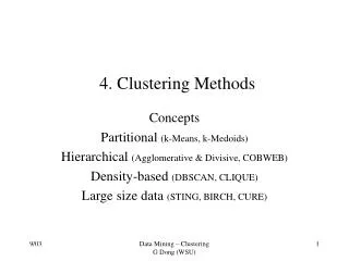
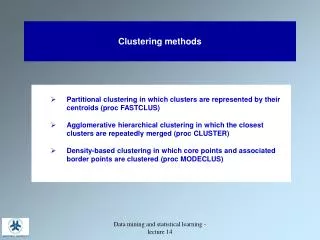
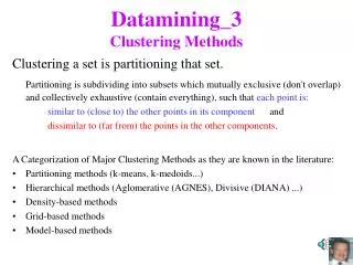
Datamining_3Clustering Methods Clustering a set is partitioning that set. Partitioning is subdividing into subsets which mutually exclusive (don't overlap) and collectively exhaustive (contain everything), such that each point is: similar to (close to) the other points in its component and dissimilar to (far from) the points in the other components. A Categorization of Major Clustering Methods as they are known in the literature: • Partitioning methods (k-means, k-medoids...) • Hierarchical methods (Aglomerative (AGNES), Divisive (DIANA) ...) • Density-based methods • Grid-based methods • Model-based methods
The k-Means Clustering Method Given k, the k-means algorithm is implemented in 4 steps (assumes partitioning criteria is: maximize intra-cluster similarity and minimize inter-cluster similarity. Of course, a heuristic is used. The method isn’t really an optimization) • Partition into k subsets (or pick k initial means). • Compute the mean (center) or centroid of each cluster of the current partition (if one started with k means initially, then this step is done). a centroid ~= a point that minimizes the sum of dissimilarities from the mean or the sum of the square errors from the mean. Assign each object to the cluster with the most similar (closest) center. • Go back to Step 2 (recompute the new centroids of the new clusters). • Stop when the new set of means doesn’t change much (or some other stopping condition?).
10 9 8 7 6 5 4 3 2 1 0 0 1 2 3 4 5 6 7 8 9 10 k-Means Clustering annimatedcentroids are red, set points are blue Step 1: assign each point to the closest centroid. Step 2: recalculate centroids. Step 3: re-assign each point to closest centroid. 10 9 8 7 6 5 4 3 2 1 0 0 1 2 3 4 5 6 7 8 9 10 Step 4: repeat 2 and 3 until Stop_Condition=true • What are the Strengths of k-Means Clustering? It is relatively efficient: O(tkn), • n is # objects, k is # clusters t is # iterations. Normally, k, t << n. • Weakness?It is applicable only when mean is defined (e.g., a vector space or similarity space). There is a need to specify k, the number of clusters, in advance. • It is sensitive to noisy data and outliers. • It can fail to converge (or converge too slowly).
The K-Medoids Clustering Method • Find representativeobjects, called medoids, (which must be an actual objects from the set, where as the means seldom are points in the set itself). • PAM (Partitioning Around Medoids, 1987) • Choose an initial set of k medoids. • Iteratively replace one of the medoids by a non-medoid. • If it improves the aggregate similarity measure, retain the replacement. Do this over all medoid-nonmedoid pairs. • PAM works for small data sets, but it does not scale well to large data sets. • Later Modifications of PAM: • CLARA (Clustering LARge Applications) (Kaufmann,Rousseeuw, 1990) Sub-samples then applies PAM. • CLARANS (Clustering Large Applications based on RANdom Search) (Ng & Han, 1994): Randomized the sampling of CLARA.
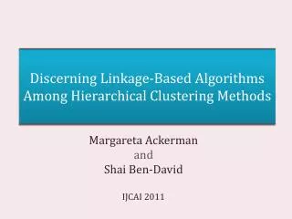
Hierarchical Clustering Methods: AGNES (Agglomerative Nesting) • Introduced in Kaufmann and Rousseeuw (1990) • Uses the Single-Link set distance (distance between two sets the minimum pairwise distance). • Other options are • complete link (distance is maximum pairwise distance); • average link • ... • Starting with each point being a cluster component of its own, itteratively merge the two clusters that are most similarity. Retain each new clustering in a hierarchy. • Eventually all nodes belong to the same cluster at the top or root node of this hierarchy or tree.
DIANA (Divisive Analysis) • Introduced in Kaufmann and Rousseeuw (1990) • Reverse AGNES (initially all objects are in one cluster; then itteratively split cluster components into two components according to some criteria (e.g., maximize some aggregate measure of pairwise dissimilarity again) • Eventually each node forms a cluster on its own
Contrasting DIANA and AGNES top down (divisively). bottom up (agglomerative)
Agglomerative a Step 1 Step 2 Step 3 Step 4 Step 0 a b b a b c d e c c d e d d e e Another look at Hierarchical Clustering
a a b b a b c d e c c d e d d e e Divisive Step 3 Step 2 Step 1 Step 0 Step 4 Another look at Hierarchical Clustering In either case, one gets a nice dendogram in which any maximal anti-chain (no 2 nodes are linked) is a clustering.
Hierarchical Clustering (Cont.) Any maximal anti-chain (maximal set of nodes in which no 2 are directly connected) is a clustering (a dendogram offers many).
Hierarchical Clustering (Cont.) But the “horizontal” anti-chains are the clusterings resulting from the top down (or bottom up) method(s).
Data Mining Summary Data Mining on a given table of data includes Association Rule Mining (ARM) on Bipartite Relationships Clustering Partitioning methods (K-means | K-medoids...), Hierarchical methods (Agnes, Diana...), Model-based methods (K-Means, K-Medoids..), .... Classification Decision Tree Induction, Bayesian, Neural Network, k-Nearest-Neighbor,...) But most data mining is on a database, not just one table, that is, often times, first one must apply the appropriate SQL query to a database to get the table to be data mined. The next slides discuss vertical data methods for doing that. You may wish to skip this material if not interested in the topic.
Partition tree R / … \ C1 … Cn /…\ … /…\ C11…C1,n1Cn1…Cn,nn . . . Vertical, compressed, lossless structures that facilitates fast horizontal AND-processing Formally, P-trees are be defined as any of the following; Partition-tree: Tree of nested partitions (a partition P(R)={C1..Cn}; each component of which is partitioned by P(Ci)={Ci,1..Ci,ni} i=1..n; each component of which is partitioned by P(Ci,j)={Ci,j1..Ci,jnij}, etc. Review of Ptrees Predicate-tree: For a predicate on the leaf-nodes of a partition-tree (also induces predicates on i-nodes using quantifiers) Predicate-tree nodes can be truth-values (Boolean P-tree); can be quantified existentially (1 or a threshold %) or universally; Predicate-tree nodes can count # of true leaf children of that component (Count P-tree). Purity-tree: universally quantified Boolean-Predicate-tree (e.g., if the predicate is <=1>, Pure1-tree or P1tree) A 1-bit at a node iff corresponding component is pure1 (universally quantified) There are many other useful predicates, e.g., NonPure0-trees; But we will focus on P1trees. All Ptrees shown so far were: 1-dimensional (recursively partition by halving bit files), but they can be; 2-D (recursively quartering) (e.g., used for 2-D images); 3-D (recursively eighth-ing), …; Or based on purity runs or LZW-runs or … Further observations about Ptrees: Partition-tree: have set nodes Predicate-tree: have either Boolean nodes (Boolean P-tree)or count nodes (Count P-tree) Purity-tree: being universally quantified Boolean-Predicate-tree have Boolean nodes (since the count is always the “full” count of leaves, expressing Purity-trees as count-trees is redundant. Partition-tree can be sliced at a level if each partition is labeled with same label set (e.g., Month partition of years). A Partition-tree can be generalized to a Set-graph when the siblings of a node do not form a partition.
Vertical Select-Project-Join (SPJ) Queries S|s____|name_|gen|C|c____|name|st|term| E|s____|c____|grade | |0 000|CLAY |M 0||0 000|BI |ND|F 0| |0 000|1 001|B 10| |1 001|THAIS|M 0||1 001|DB |ND|S 1| |0 000|0 000|A 11| |2 010|GOOD |F 1||2 010|DM |NJ|S 1| |3 011|1 001|A 11| |3 011|BAID |F 1||3 011|DS |ND|F 0| |3 011|3 011|D 00| |4 100|PERRY|M 0||4 100|SE |NJ|S 1| |1 001|3 011|D 00| |5 101|JOAN |F 1||5 101|AI |ND|F 0| |1 001|0 000|B 10| |2 010|2 010|B 10| |2 010|3 011|A 11| |4 100|4 100|B 10| |5 101|5 101|B 10| A Select-Project-Join query has joins, selections and projections. Typically there is a central fact relation to which several dimension relations are to be joined (standard STAR DW) E.g., Student(S), Course(C), Enrol(E) STAR DB below (bit encoding is shown in reduced font italics for certain attributes) Vertical bit sliced (uncompressed) attrs stored as: S.s2S.s1S.s0S.gC.c2C.c1C.c0C.tE.s2E.s1E.s0E.c2E.c1E.c0E.g1 E.g0 0 0 0 0 0 0 0 00 0 0 0 0 1 1 0 0 0 1 0 0 0 1 10 0 0 0 0 0 1 1 1 0 0 0 1 0 0 10 0 1 0 1 1 0 0 1 0 1 1 1 0 1 00 0 1 0 0 0 1 0 0 1 0 1 0 1 0 10 1 1 0 1 1 1 1 0 1 1 1 0 1 1 00 1 1 0 1 1 0 0 0 1 0 0 1 0 1 0 0 1 0 0 0 1 1 1 1 0 0 1 0 0 1 0 1 0 1 1 0 1 1 0 Vertical (un-bit-sliced) attributes are stored:S.name C.nameC.st |CLAY ||BI | |ND| |THAIS||DB | |ND| |GOOD ||DM | |NJ| |BAID ||DS | |ND| |PERRY||SE | |NJ| |JOAN ||AI | |ND|
Vertical preliminary Select-Project-Join Query Processing (SPJ) decimal binary. In the SCORE database (Students, Courses, Offerings, Rooms, Enrollments), numeric attributes are represente vertically as P-trees (not compressed). Categorical are projected to a 1 column vertical file SELECTS.n, C.nFROMS, C, O, R, E WHERES.s=E.s&C.c=O.c&O.o=E.o&O.r=R.r &S.g=M&C.r=2&E.g=A&R.c=20; R:r cap |0 00|30 11| |1 01|20 10| |2 10|30 11| |3 11|10 01| R.r1 0 0 1 1 R.r0 0 1 0 1 R.c1 1 1 1 0 R.c0 1 0 1 1 S:s ngen |0 000|A|M| |1 001|T|M| |2 100|S|F| |3 111|B|F| |4 010|C|M| |5 011|J|F| S.s2 0 0 1 1 0 0 S.s1 0 0 0 0 1 1 S.s0 0 1 0 1 0 1 S.n A T S B C J S.g M M F F M F O.o2 0 0 0 0 1 1 1 1 O :o c r |0 000|0 00|0 01| |1 001|0 00|1 01| |2 010|1 01|0 00| |3 011|1 01|1 01| |4 100|2 10|0 00| |5 101|2 10|2 10| |6 110|2 10|3 11| |7 111|3 11|2 10| O.o1 0 0 1 1 0 0 1 1 O.o0 0 1 0 1 0 1 0 1 O.c1 0 0 0 0 1 1 1 1 O.c0 0 0 1 1 0 0 0 1 O.r1 0 0 0 0 0 1 1 1 O.r0 1 1 0 1 0 0 1 0 E:s o grade |0 000|1 001|2 10| |0 000|0 000|3 11| |3 011|1 001|3 11| |3 011|3 011|0 00| |1 001|3 011|0 00| |1 001|0 000|2 10| |2 010|2 010|2 10| |2 010|7 111|3 11| |4 100|4 100|2 10| |5 101|5 101|2 10| E.s2 0 0 0 0 0 0 0 0 1 1 E.s1 0 0 1 1 0 0 1 1 0 0 E.s0 0 0 1 1 1 1 0 0 0 1 E.o2 0 0 0 0 0 0 0 1 1 1 E.o1 0 0 0 1 1 0 1 1 0 0 E.o0 1 0 1 1 1 0 0 1 0 1 E.g1 1 1 1 0 0 1 1 1 1 1 E.g0 0 1 1 0 0 0 0 1 0 0 C.c0 0 1 0 1 C.n B D M S C.r0 1 1 1 0 C.c1 0 0 1 1 C.r1 0 1 1 1 C:c ncred |0 00|B|1 01| |1 01|D|3 11| |2 10|M|3 11| |3 11|S|2 10|
S.s2 0 0 1 1 0 0 S.s1 0 0 0 0 1 1 S.s0 0 1 0 1 0 1 S.n A T S B C J SM 1 1 0 0 1 0 S.g 1 1 0 0 1 0 O.o2 0 0 0 0 1 1 1 1 O.o1 0 0 1 1 0 0 1 1 O.o0 0 1 0 1 0 1 0 1 O.c1 0 0 0 0 1 1 1 1 O.c0 0 0 1 1 0 0 0 1 O.r1 0 0 0 0 0 1 1 1 O.r0 1 1 0 1 0 0 1 0 R.r1 0 0 1 1 R.r0 0 1 0 1 R.c1 1 1 1 0 R.c1 1 1 1 0 R.c0 1 0 1 1 R.c’0 0 1 0 0 E.s2 0 0 0 0 0 0 0 0 1 1 E.s1 0 0 1 1 0 0 1 1 0 0 E.s0 0 0 1 1 1 1 0 0 0 1 E.o2 0 0 0 0 0 0 1 0 1 1 E.o1 0 0 0 1 1 0 1 1 0 0 E.o0 1 0 1 1 1 0 0 1 0 1 E.g1 1 1 1 0 0 1 1 1 1 1 E.g1 1 1 1 0 0 1 1 1 1 1 E.g0 0 1 1 0 0 0 0 1 0 0 E.g0 0 1 1 0 0 0 0 1 0 0 EgA 0 1 1 0 0 0 0 1 0 0 C.c1 0 0 1 1 C.n B D M S C.c1 0 1 0 1 C.r1 0 1 1 1 C.r1 0 1 1 1 C.r’2 0 0 0 1 C.r2 1 1 1 0 Rc20 0 1 0 0 Cr2 0 0 0 1 For selections, S.g=M=1bC.r=2=10bE.g=A=11bR.c=20=10b create the selection masks using ANDs and COMPLEMENTS. Apply these selection masks (Zero out numeric values, blanked out others). S.s2 0 0 0 0 0 0 S.s1 0 0 0 0 1 0 S.s0 0 1 0 0 0 0 S.n A T C O.o2 0 0 0 0 1 1 1 1 O.o1 0 0 1 1 0 0 1 1 0 0 1 0 1 0 1 0 1 O.c1 0 0 0 0 1 1 1 1 O.c0 0 0 1 1 0 0 0 1 O.r1 0 0 0 0 0 1 1 1 O.r0 1 1 0 1 0 0 1 0 R.r1 0 0 0 0 R.r0 0 1 0 0 E.s2 0 0 0 0 0 0 0 0 0 0 E.s1 0 0 1 0 0 0 0 1 0 0 E.s0 0 0 1 0 0 0 0 0 0 0 E.o2 0 0 0 0 0 0 0 1 0 0 E.o1 0 0 0 0 0 0 0 1 0 0 E.o0 0 0 1 0 0 0 0 1 0 0 C.c1 0 0 0 1 C.n S C.c0 0 0 0 1 SELECTS.n, C.nFROMS, C, O, R, E WHERES.s=E.s&C.c=O.c&O.o=E.o&O.r=R.r &S.g=M&C.r=2&E.g=A&R.c=20;
S.s2 0 0 0 0 0 0 S.s1 0 0 0 0 1 0 S.s0 0 1 0 0 0 0 S.n A T C O.o2 0 0 0 0 1 1 1 1 O.o1 0 0 1 1 0 0 1 1 O.o0 0 1 0 1 0 1 0 1 O.c1 0 0 0 0 1 1 1 1 O.c0 0 0 1 1 0 0 0 1 O.r1 0 0 0 0 0 1 1 1 O.r1 0 0 0 0 0 1 1 1 O.r0 1 1 0 1 0 0 1 0 O’.r0 0 0 1 0 1 1 0 1 R.r1 0 0 0 0 R.r0 0 1 0 0 Rc20 0 1 0 0 E.s2 0 0 0 0 0 0 0 0 0 0 E.s1 0 0 1 0 0 0 0 1 0 0 E.s0 0 0 1 0 0 0 0 0 0 0 E.o2 0 0 0 0 0 0 0 1 0 0 E.o1 0 0 0 0 0 0 0 1 0 0 E.o0 0 0 1 0 0 0 0 1 0 0 C.c1 0 0 0 1 C.n S C.c0 0 0 0 1 For the joins, S.s=E.sC.c=O.cO.o=E.oO.r=R.r,one approach is to follow an indexed nested loop like method. (Noting that attribute P-trees ARE an index for that attribute). The join O.r=R.ris simply part of a selection on O (R doesn’t contribute output nor participate in any further operations) Use the Rc20-masked R as the outer relation Use O as the indexed inner relation to produce that O-selection mask. Get 1st R.r value, 01b (there's only 1) Mask the O tuples: PO.r1^P’O.r0 OM 0 0 0 0 0 1 0 1 O.o2 0 0 0 0 0 1 0 1 O.o1 0 0 0 0 0 0 0 1 O.o0 0 0 0 0 0 1 0 1 O.c1 0 0 0 0 0 1 0 1 O.c0 0 0 0 0 0 0 0 1 This is the only R.r value (if there were more, one would do the same for each, then OR those masks to get the final O-mask). Next, we apply the O-mask, OM to O SELECTS.n, C.nFROMS, C, O, R, E WHERES.s=E.s&C.c=O.c&O.o=E.o&O.r=R.r &S.g=M&C.r=2&E.g=A&R.c=20;
O.o2 0 0 0 0 0 1 0 1 O.o1 0 0 0 0 0 0 0 1 O.o0 0 0 0 0 0 1 0 1 O.c1 0 0 0 0 0 1 0 1 O.c1 0 0 0 0 0 1 0 1 O.c0 0 0 0 0 0 0 0 1 O.c0 0 0 0 0 0 0 0 1 E.s2 0 0 0 0 0 0 0 0 0 0 E.s1 0 0 1 0 0 0 0 1 0 0 E.s0 0 0 1 0 0 0 0 0 0 0 E.o2 0 0 0 0 0 0 0 1 0 0 E.o2 0 0 0 0 0 0 0 1 0 0 E.o1 0 0 0 0 0 0 0 1 0 0 E.o1 0 0 0 0 0 0 0 1 0 0 E.o0 0 0 1 0 0 0 0 1 0 0 E.o0 0 0 1 0 0 0 0 1 0 0 S’.s2 1 1 0 0 1 0 S.s2 0 0 0 0 0 0 S.s1 0 0 0 0 1 0 S.s1 0 0 0 0 1 0 S’.s0 1 0 0 0 1 0 S.s0 0 1 0 0 0 0 S.n A T C C.c1 0 0 0 1 C.c0 0 0 0 1 C.n S For the final 3 joins C.c=O.cO.o=E.o E.s=S.sthe same indexed nested loop like method can be used. OM 0 0 0 0 0 0 0 1 EM 0 0 0 0 0 0 0 1 0 0 Get 1st masked C.c value, 11b Mask corresponding O tuples: PO.c1^PO.c0 Get 1st masked O.o value, 111b Mask corresponding E tuples: PE.o2^PE.o1^PE.o0 SM 0 0 0 0 1 0 Get 1st masked E.s value, 010b Mask corresponding S tuples: P’S.s2^PS.s1^P’S.s0 Get S.n-value(s), C, pair it with C.n-value(s), S, output concatenation, C.nS.n S C There was just one masked tuple at each stage in this example. In general, one would loop through the masked portion of the extant domain at each level (thus,Indexed Horizontal Nested Loop or IHNL) SELECTS.n, C.nFROMS, C, O, R, E WHERES.s=E.s&C.c=O.c&O.o=E.o&O.r=R.r &S.g=M&C.r=2&E.g=A&R.c=20;
Vertical Select-Project-Join-Classification Query Given previous SCORE Training Database (not presented as just one training table), predict what course a male student will register for, who got an A in a previous course in Room with a capacity of 20. This is a matter of applying the previous complex SPJ query first to get the pertinent Training table and then classifying the above unclassified sample (e.g., using, 1-nearest neighbour classification). The result of the SPJ is the single row Training Set, (S,C) and so the prediction is course=C.