Clustering Methods for Class Discovery

1. Clustering Methods for Class Discovery

2. Introduction

3. Gene expression profiles • Many genes show definite changes of expression between conditions • These patterns are called gene profiles

4. Motivation (1): The problem of finding patterns • It is common to have hybridizations where conditions reflect temporal or spatial aspects. • Yeast cycle data • Tumor data evolution after chemotherapy • CNS data in different part of brain • Interesting genes may be those showing patterns associated with changes. • Our problem seems to be distinguishing interesting or real patterns from meaningless variation, at the level of the gene

5. Finding patterns: Two approaches • If patterns already exist  Profile comparison (Distance analysis) • Find the genes whose expression fits specific, predefined patterns. • Find the genes whose expression follows the pattern of predefined gene or set of genes. • If we wish to discover new patterns Cluster analysis (class discovery) • Carry out some kind of exploratory analysis to see what expression patterns emerge;

6. Motivation (2): Tumor classification • A reliable and precise classification of tumours is essential for successful diagnosis and treatment of cancer. • Current methods for classifying human malignancies rely on a variety of morphological, clinical, and molecular variables. • In spite of recent progress, there are still uncertainties in diagnosis. Also, it is likely that the existing classes are heterogeneous. • DNA microarrays may be used to characterize the molecular variations among tumours by monitoring gene expression on a genomic scale. This may lead to a more reliable classification of tumours.

7. Tumor classification, cont • There are three main types of statistical problems associated with tumor classification: • The identification of new/unknown tumor classes using gene expression profiles - cluster analysis; • The classification of malignancies into known classes - discriminant analysis; • The identification of “marker” genes that characterize the different tumor classes - variable selection.

8. Cluster and Discriminant analysis • These techniques group, or equivalently classify, observational units on the basis of measurements. • They differ according to their aims, which in turn depend on the availability of a pre-existing basis for the grouping. • In cluster analysis (unsupervised learning, class discovery) , there are no predefined groups or labels for the observations, • Discriminant analysis(supervised learning, class prediction) is based on the existence of groups (labels)

9. Clustering microarray data • Cluster can be applied to genes (rows), mRNA samples (cols), or both at once. • Cluster samples to identify new cell or tumour subtypes. • Cluster rows (genes) to identify groups of co-regulated genes. • We can also cluster genes to reduce redundancy e.g. for variable selection in predictive models.

10. Advantages of clustering • Clustering leads to readily interpretable figures. • Clustering strengthens the signal when averages are taken within clusters of genes (Eisen). • Clustering can be helpful for identifying patterns in time or space. • Clustering is useful, perhaps essential, when seeking new subclasses of cell samples (tumors, etc).

11. Applications of clustering (1) • Alizadeh et al (2000) Distinct types of diffuse large B-cell lymphoma identified by gene expression profiling. • Three subtypes of lymphoma (FL, CLL and DLBCL) have different genetic signatures. (81 cases total) • DLBCL group can be partitioned into two subgroups with significantly different survival. (39 DLBCL cases)

12. Clusters on both genes and arrays Taken from Nature February, 2000 Paper by Allizadeh. A et al Distinct types of diffuse large B-cell lymphoma identified by Gene expression profiling,

13. Discovering tumor subclasses • DLBCL is clinically heterogeneous • Specimens were clustered based on their expression profiles of GC B-cell associated genes. • Two subgroups were discovered: • GC B-like DLBCL • Activated B-like DLBCL

14. Applications of clustering (2) • A naïve but nevertheless important application is assessment of experimental design • If one has an experiment with different experimental conditions, and in each of them there are biological and technical replicates… • We would expect that the more homogeneous groups tend to cluster together • Tech. replicates < Biol. Replicates < Different groups • Failure to cluster so suggests bias due to experimental conditions more than to existing differences.

15. Basic principles of clustering

16. Basic principles of clustering Aim: to group observations that are “similar” based on predefined criteria. Issues: Which genes / arrays to use? Which similarity or dissimilarity measure? Which clustering algorithm? • It is advisable to reduce the number of genes from the full set to some more manageable number, before clustering. The basis for this reduction is usually quite context specific, see later example.

17. Two main classes of measures of dissimilarity • Correlation • Distance • Manhattan • Euclidean • Mahalanobis distance • Many more ….

18. Two basic types of methods Hierarchical Partitioning

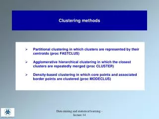
19. Partitioning methods Partition the data into a pre-specified numberk of mutually exclusive and exhaustive groups. Iteratively reallocate the observations to clusters until some criterion is met, e.g. minimize within cluster sums of squares. Examples: • k-means, self-organizing maps (SOM), PAM, etc.; • Fuzzy: needs stochastic model, e.g. Gaussian mixtures.

20. Hierarchical methods • Hierarchical clustering methods produce a tree or dendrogram. • They avoid specifying how many clusters are appropriate by providing a partition for each k obtained from cutting the tree at some level. • The tree can be built in two distinct ways • bottom-up: agglomerative clustering; • top-down: divisive clustering.

21. Agglomerative methods • Start with n clusters. • At each step, merge the two closest clusters using a measure of between-cluster dissimilarity, which reflects the shape of the clusters. • Between-cluster dissimilarity measures • Mean-link: average of pairwise dissimilarities • Single-link: minimum of pairwise dissimilarities. • Complete-link: maximum& of pairwise dissimilarities. • Distance between centroids

22. Distance between centroids Single-link Mean-link Complete-link

23. Divisive methods • Start with only one cluster. • At each step, split clusters into two parts. • Split to give greatest distance between two new clusters • Advantages. • Obtain the main structure of the data, i.e. focus on upper levels of dendogram. • Disadvantages. • Computational difficulties when considering all possible divisions into two groups.

24. 4 1 5 2 3 Illustration of points In two dimensional space Agglomerative 1,2,3,4,5 4 3 1,2,5 3,4 5 1,5 1 2 1 5 2 3 4

25. Tree re-ordering? 4 1 5 2 3 Agglomerative 2 1 5 3 4 1,2,3,4,5 4 3 1,2,5 3,4 5 1,5 1 2 1 5 2 3 4

26. Partitioning: Advantages Optimal for certain criteria. Genes automatically assigned to clusters Disadvantages Need initial k; Often require long computation times. All genes are forced into a cluster. Hierarchical Advantages Faster computation. Visual. Disadvantages Unrelated genes are eventually joined Rigid, cannot correct later for erroneous decisions made earlier. Hard to define clusters. Partitioning or Hierarchical?

27. Hybrid Methods • Mix elements of Partitioning and Hierarchical methods • Bagging • Dudoit & Fridlyand (2002) • HOPACH • van der Laan & Pollard (2001)

28. Three generic clustering problems Three important tasks (which are generic) are: 1. Estimating the number of clusters; 2. Assigning each observation to a cluster; 3. Assessing the strength/confidence of cluster assignments for individual observations. Not equally important in every problem.

29. Estimating number of clusters using silhouette • Define silhouette width of the observation as : S = (b-a)/max(a,b) • Where a is the average dissimilarity to all the points in the cluster and b is the minimum distance to any of the objects in the other clusters. • Intuitively, objects with large S are well-clustered while the ones with small S tend to lie between clusters. • How many clusters: Perform clustering for a sequence of the number of clusters k and choose the number of components corresponding to the largest average silhouette. • Issue of the number of clusters in the data is most relevant for novel class discovery, i.e. for clustering samples

30. Estimating number of clusters using the bootstrap There are other resampling (e.g. Dudoit and Fridlyand, 2002) and non-resampling based rules for estimating the number of clusters (for review see Milligan and Cooper (1978) and Dudoit and Fridlyand (2002) ). The bottom line is that none work very well in complicated situation and, to a large extent, clustering lies outside a usual statistical framework. It is always reassuring when you are able to characterize a newly discovered clusters using information that was not used for clustering.

31. Limitations • Usually outside the normal framework of statistical inference; • less appropriate when only a few genes are likely to change. • Needs lots of experiments • Always possible to cluster even if there is nothing going on. • Useful for learning about the data, but does not provide biological truth.

32. Some examples using R

33. The data • We will use the dataset presented in van't Veer et al.  (2002) which is available at http://www.rii.com/publications/2002/vantveer.htm. • These data come from a study of gene expression in 91 breast cancer node-negative tumors. • The training samples consisted of 78 tumors, 44 of which did not recur within 5 years of diagnosis and 34 did. • Among the test samples, 7 have not recurred within 5 years and 12 did. • The data were collected on two color Agilent oligo arrays containing about 24K genes..

34. Preprocessing • The data has been filtered using procedures described in the original manuscript. • Only genes showing 2-fold differential expression and p-value for a gene being expressed < 0.01 in more than 5 samples are retained. • There are 4,348 such genes. • Missing values were imputed using k-nearest neighbors imputation procedure (Troyanskaya, et al, 2001). • There, for each gene containing at leats one missing value we find 5 genes most highly correlated with it and take average of their value for the sample in which a value for a given gene is missing. • The missing value is replaced with the average.

35. R data • The filtered gene expression levels  are stored in a 4348 × 97 matrix named bcdata with rows corresponding to genes and columns to mRNA samples. • Additionally, the labels are contained in the 97-element vector surv.resp with 0 indicating good outcome (no recurrence within 5 years after diagnosis) and 1 indicating bad outcome (recurrence within 5 years after diagnosis).

36. Start performing a hierarchical clustering on the mRNA samples using correlation as similarity function and complete linkage agglomeration library(stats) x1<-as.dist(1 - cor(bcdata) clust.cor <- hclust(x1), method="complete") plot(clust.cor, cex = 0.6) Hierarchical clustering (1)

37. Hierarchical clustering (1)

38. Perform a hierarchical clustering on the mRNA samples using Euclidean distance and average linkage agglomeration. Results can differ significantly. X2<-dist(t(bcdata) clust.euclid <- hclust(x2), method = "average") plot(clust.euclid, cex = 0.6) Hierarchical clustering (2)

39. Hierarchical clustering (2)

40. Comparison between orderings • IN THIS CASE WE OBSERVE THAT: • Clustering based on correlation and complete linkage dsitributes samples more uniformly between groups • Euclidean-average linkage combination yields one huge group and many small one

41. If we assume a fixed number of clusters we can use a partitioning method such as PAM It is a robust version of k-means which clusters data around the medoids Partitioning around medoids library(cluster) x3<-as.dist(1-cor(bcdata)) clust.pam <- pam(x3, 5, diss =TRUE) clusplot(clust.pam, labels = 5, col.p = clust.pam$clustering)

42. PAM clustering (2)