Download

1 / 37
380 likes | 466 Vues
Understand central concepts like sampling error, null hypothesis, standard error, degrees of freedom, and more in inferential statistics. Learn about one-tailed and two-tailed tests, effect size, and significance levels. Explore examples and implications of statistical tests.

E N D
Inferential statistics PSY 4010
Central concepts in inferential statistics: • Sampling error • Sampling distribution • Standard error • Null hypothesis and alternative hypothesis • Level of significance • Type I and Type II error • One-tailed and two-tailed tests • Degrees of freedom • Parametric and non-parametric statistical tests • Effect size
Sample and population Population Sample
Example: IQ-mean score in population and sample • The population mean IQ-score equals 100 (=100) and the standard deviation is 15 ( = 15) • You draw three samples consisting of 25 randomly selected persons from this population and estimates the mean IQ score in each sample : Sample 1: 103 Sample 2 101 Sample 3 98 Sampling error (coincidence results in deviation from population mean score) 103-100 = 3 101-100 = 1 98-100 = -2
Sampling distribution and standard error • Sampling distribution: • Distribution of the mean values of an infinitive number of samples of the same size drawn from the same population • Can also be other measures then mean values, e.g. Correlation coefficients, regression coefficients • The standard deviation of such a sampling distribution is called the standard error • A very important measure, an estimate of variability in mean scores due to chance (sampling error)
Standard error • The standard error is a function of two things: • : How large the standard deviation in the population is • N: The size of the sample Examples based on samples drawn from a population with a standard deviation() of 15 (and mean of 100) • N = 9 • N = 25 • N = 100
N = 100 N = 9 Sampling distribution at different sample sizes Infinitive number of samples randomly drawn from a population with = 100 and standard deviation = 15 N = 25 85 90 95 100 105 110 115
13,6% 34,1% 34,1% 13,6% 2,2 % 0,1 % 0,1 % 2,2 % Sampling distribution and standard error 50 % of the samples mean values is under the population mean 50 % is over -3 X -2 X -1 X +1 X +2 X +3 X
Example: IQ and breast-feeding • The population mean score on IQ for 12 years old is 100 and the standard deviation is 15 • A researcher suspects that breast-feeding can affect IQ • A sample of 25 12-year olds being breast-fed up to six months of age have a mean IQ-score of 103 • How probable is it that this sample has = 103 due to sampling error?
Testing hypotesis Null hypothesis (H0): The population of children being breast-fed up to 6 months of age does not have a different mean IQ score from other children I.e.: the difference from the population mean score is due to sampling error Alternative hypothesis (H1): The population of children being breast-fed up to 6 mnds of age does have a different mean IQ score from the population of other children How probable is it to obtain a difference of 3 points or more in mean score due to sampling error/pure chance? This is referred to as the p-value
13,6% 34,1% 34,1% 13,6% 2,2 % 0,1 % 0,1 % 2,2 % Sampling distribution when the standard error equals 3 Sample = 103 -3 X -2 X -1 X +1 X +2 X +3 X 91 94 97 100 103 106 109
How probable is it that the results is due to random variation (sampling error)? In our example: a of 103 or higher will appear in 15,9 % (p= 0.159) of all the N = 25 samples we draw from a population with =100, = 15 Thus, the probability of sampling error is 15,9 %
Significance level The limit we set in order to reject H0 is called significance level () : • Convention: if the probability sampling error is less than5 %, we reject the Null hypothesis. • If the probability of sampling error is 5 % or more, keep H0 • We usually symbolize this as = 0.05 • We can also set the level to 1 % or lower ( = 0.01) • Based on the results, we…….keep H0
One-tailed and two-tailed tests • A one-tailed test: the difference is in an expected direction: H0 : (The population) of children who are breast-fed up to 6 mnds of age have higher mean IQ-score than other children • A two-tailed test H1 : (The population) of children who are breast-fed up to 6 mnds of age have a different mean IQ-score than other children (Thus, we open up for the possibility that the mean IQ-score of breast-fed children can be either lower or higher than in the population of other children) • Important to decide upon one- ore two-tailed test before the test is conducted!
Consequences of choosing a one-tailed or a two-tailed test One-tailed Two-tailed Rejection area 1.65 1.96 -1.96 Critical value
Task 1 We now have increased our a sample to 100 children who have been breast-fed up to 6 mnds of age. The sample’s mean score on IQ is the same: 103 If you choose a level of significance of 5 % ( = .05), do you reject or keep H0?
Type I and Type II error We can never be 100% sure that we do the right thing when rejecting or keeping H0: THUS: We do not say that H0 is true or false, or that H1 is so.
We use the sample’s standard deviation (s) as an estimate of the population‘s standard deviation () Standard error if we know population standard deviance: Standard error if we do not know population standard deviance: In practice: (small) samples often underestimate the standard deviation in the population Therefore, this is taken into consideration in the test for significance applied Most applied; the student t-distribution What do we do when we do not know the population values?
The Student t distribution is different for different sample sizes Sample sizes are represented as the degrees of freedom (df) df = N -1 A sample of 10 has (10-1) = 9 degrees of freedom Must take this into consideration The more degrees of freedom, the more identical to the Z-distribution the Student t distribution will be The Student t distribution
The t distribution Different samples sizes (df) have different critical values
Example: do drivers’ mean speed deviate from the speed limit when it is raised to 100 km/h on a road section? You measured the speed of 30 cars. These have: H0: µ = 100 H1: µ ≠ 100 What is the critival value for rejecting H0at a 5 % level? df = N-1 = 30-1 = 29 When the population’s standard deviation is not known
The t distribution For a two-tailed test with 5 % level of significance and 29 df, The critical value is +/- 2.045
-5,47 -2,045 2,045 Our estimated t-value is in the rejection area, and we reject H0 Thus, we believe that the real driving speed is below 100 km/h
Difference in mean score between two samples, no information about population values Is the difference between the experimental group (N =8) and control group (N =8) on mean depression score after treatment statistically significant? Null hypothesis (H0): Alternative hypothesis (H1): How probable is it that the difference in due to sampling error?
-2,629 H0 is rejected, we believe that the difference between the experimental group and the control group is present in the population i.e.: training seems to work! -2,145 2,145
Degrees of freedom (df): Nexp.group -1 + Ncontrol group -1 = 8-1 + 8-1 = 14 Critcal value for a two-tailed test df = 14, = 0.05: +/- 2.145
Parametric tests • Parametric tests are based upon three main assumptions • The sample(s) is randomly drawn from the population • The values are normally distributed in the population • If two or more samples are compared to each other, they must be drawn from populations with equal variances This are very rigid assumption. However, parametric tests are quite robust to violation of assumption 2 and 3
Examples of parametric tests Applied when we know the population values (mean score, standard deviation, or percentage etc.) • Z-test Applied when we do not know the population values • t-test (difference in mean scores between groups, correlation and regression coefficients) • F-test (Analysis of variance)
Non-parametric tests • Applied when assumptions of parametric tests are violated • Or when dependent variables are on a ordinal/nominal level • Basically the same logic is applied as for significance testing using parametric tests
Example of a non-parametric test: the chi-square test (2) • Is being found guilty or not for violent crimes dependent upon skin color? • Both variables are measured on a nominal level, and mean and standard deviation cannot be estimated • In this case we use the chi-square test (2) to determine whether the difference is significant or not
Core of the chi-square test Calculate the expected values (E) which symbolize the values if there were no relationship between the two variables • Compare these to the observed values (O) using this formula:
We must also estimate the number of freedom: df = (the number of columns -1) + (the number of rows-1) df = (2-1) + (2-1) = 1 • And next find the critical value of 2 at a 5 % level of significance • H0: there is no association between skin color and being found guilty • H1: there is an association between skin color and being found guilty
The 2 distribution The critical value of 2 (df =1) = 3.84 Our estimated 2 value is 32, thus much larger than 3.84 Thus, H0is rejected
Level of significance and practical importance/significance • A statistical significant result is not necessary of large practical importance • The main reason: statistical significant result is strongly influenced by the size of the sample(s) • Large samples = easy to obtain significant results (i.e. easier to reject H0) • Small samples = difficult to obtain significant results • Useful to include a measure of effect size also • Focusing on how large the difference is/ how strong the association between the variables are
Several types: For differences in mean D-value: (difference relative to standard deviation) Interpretation of d d= 0, no difference +/- 0.20: small difference +/- 0.50: moderate difference +/- .80: large difference For measures of association and explained variance: r, r2 and R2 Eta2 Effect size
Random sampling 1.Simple randomized sampling • All members of the population have an equal chance of being drawn 2. Systematic sampling • Selected using a certain key • E.g.. Each 50th person over 18 year 3. Stratified randomized sampling Random selection within subgroups of the population 4. Proportionate sampling. Drawing certain proportions of the sample from subgroups of the population 5. Cluster sampling. Drawing all members of randomly selected groups from the population (e.g. school classes)
Non-random samples 1.Convenience sampling • Students attending a lecture, stopping people on the street, voluntary participants 2. Quota sampling • Recruit volunteers, but make sure that certain characteristics are represented in certain proportions (e.g. equal number of each gender, age etc.)