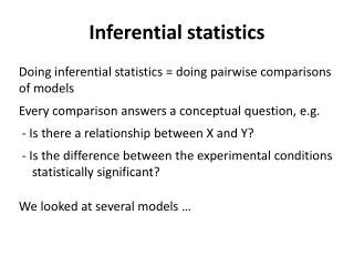
Inferential Statistics

1. Inferential Statistics Doing stats with confidence

2. Greek symbols everywhere

3. Greek symbols everywhere • Population: the total set of items that we are concerned about  • Parameter: a measure used to summarize a population (could include mean, median, standard deviation) • Sample: a subset of the population (assumed to be sampled randomly, where every object has an equally likelihood of being selected) • Statistic: a measure used to summarize a sample (mean, median, SD)

4. Calculating parameters: Populations • -Mean is always the same • -Standard deviation

5. Calculating statistics: samples • -Mean is always the same • The difference is that here you divide by (n-1) • When you only divide by N, you get consistently low estimates of the population SD sigma  • For this reason, the estimate is always made with (n-1)

6. Central Limit Theorem The most important thing in stats

7. Intuitive explanation -we can start out with any distribution (a continuous or a discrete distribution), and if it has a mean and a standard deviation, even if it looks nothing like a normal distribution:

8. Now, we take a sample from this dist. • You take a sample from this distribution (1, 2, 5, 5)  • Say the first time, you take a sample size of 4 (n=4) [a sample of 4 samples!] • The SAMPLE refers to the SET of 4 numbers, and the sample size or “n" tells you how many you took in your sample

9. Next we average this sample & Plot it • If we average out 1,2,5, and 5 we get 3.25 (then plot it) • NOW, repeat this again and again and again (i.e. increase your number of trials) and plot the mean of every single sample you take • You continue to take samples, size 4, aveerage them, plot the frequency of the averages • Say you do this 10,000 times • Your plot will begin to look like the normal distribution

10. Simulate this -Use this simulation: http://onlinestatbook.com/stat_sim/sampling_dist/

11. The simulation and what we notice about the clt • -The difference between n=5 and n=10 shows a much more normal shape, tighter around the mean • -The mean is the same between the population and the sampling distribution

12. Sampling distribution of the sample mean • This is the name of what we just made • To recap, you make it using the following steps • Take a sample size n • Average your values • Plot them • Do it over and over • Plot each one • Watch as your plot begins to approximate the normal curve

13. Standard error of the mean • When you take a sample, then take another sample, the means will be different. • When you take many samples again and again, then calculate the mean for each sample these means you can plot this to form a distribution (sampling dist. Of the sampling mean) • and then you can calculate the standard deviation of the distribution of these means • This is the standard error of the mean

14. There is a simple way to take the standard error • -you don’t even need to take 10,000 samples • s.e. is the standard error of the mean • sigma is the SD of the population • n is the sample size • But we rarely know the SD of the population  • We can use the second formula above to estimate the standard deviation 

15. Practice Problems

16. Example 1 The average woman drinks 2 L of water when active outdoors for a day (with a standard deviation of 0.7 L). You’re planning a trip for 50 women and you bring 110 L of water. What is the probability that you will run out of water?

17. Distribution of the population This data is an estimate of the population parameters. We are not told the distribution, but can guess at a drawing to ground our thinking 

18. Translate the problem into probability What we are looking for is the probability that the average woman drinks more than 2.2 liters of water (since we brought 110 L divided by 50 women)

19. Another way of saying this… • If we were to take an infinite number of samples (n=50), what is the probability of the those contained in the sample drinking more than 2.2 L • This sets us up to use the sampling distribution of the sample mean • We can take the sampling distribution of the sampling mean when n=50 • Remember, the mean would remain at 2 L

20. Calculate the standard error • We already got the mean, now we need to get the standard error • This is the same thing as the standard deviation of the sample mean = S/sqrt(n) or 0.7/sqrt(50) • Standard error = 0.099 (almost 0.1) /a very narrow SD

21. Draw your picture to conceptualize what you just found

22. Next step • Go back to the question: (we are looking for the probability our sample will have an average of 2.2 L) • our distribution is the plot of all possible samples. We will run out of water if our sample mean falls above 2.2

23. Next step • We are finding the probability of the area of under the curve highlighted in green hatching  • We can use a z table to figure out what the green area is  • When we are above 2.2 L, we are 0.2 above the mean. • If we want that in terms of standard deviations, use the formula for the z score:  • x bar - mu / sigma or (2.2-2)/0.099=0.2/0.099=2.02 • This value of 2.2 L has the same probability of being 2.02 SD above the mean

24. Look it up in the z table Be sure and consult your picture so you know exactly what your z score is telling you

25. Translate the z score into a probability

26. Final answer Final answer: there is a 2.17% chance we will run out of water (i.e. get a sample of 50 people who consume more than the mean amount of water)

27. Example 2 You sample 36 apples from your farm’s harvest of 200,000 apples. The mean weight is 112 grams (with a 40 g SD) what is the probability that the mean weight of all 200,000 apples is between 100 and 124 grams?

28. Think about what the problem wants • This is asking you to conceptualize the sampling distribution of the sample mean • We know that if we took a sample size 35 over and over, a distribution would form where the sampling mean would equal the population mean mu, and the SD of the distribution can be found with the formula for standard error

29. Start out with a picture

30. Calculate mean and s.e. • Always start by figuring out what you can: • The mean is 112 • The standard error is: 40/sqrt(36)=6.67

31. Formulate what the problem wants in terms of probability • Go back to the original question: this is asking us what the probability that the population mean is within 12 of the sample mean (x bar) • i.e. the sample mean is within 12 of the actual mean • You know you’re being asked for a confidence interval because of the range

32. Find the z score for 12 above or below the mean: • use the z score formula: x bar minus mu/ sigma • Get the z score: (112-100)/6.67=1.8 Go back to the question: This is like saying what is the probability that our sample of 36 apples is within 1.8 standard deviations of the mean?

33. Draw it again with the new information

34. Find the area under the hatching • Use the z table

35. Interpret the probability from the z table • Given this z chart shows from mean to z, you need to double it to get 1.8 SD in either direction • =0.46407*2=0.92814

36. Put it back into plain words • Put everything back in English: The probability that the sample mean is 1.8 SD from the actual mean has a 92.8 % chance, or • there is a 92.82% chance that the actual population mean is within 12 grams of our sample (between 112 & 124) • Also we are 92.8% confident that the mean is between 112 and 124 g