Designing of Cellular Mobile Networks Using Modern Heuristics

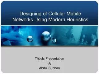
1. Designing of Cellular Mobile Networks Using Modern Heuristics Thesis Presentation By Abdul Subhan

2. Outline • Introduction • Background • Problem Description • Implementation Approach • Experimental Analysis & Results • Conclusion & Future Work

3. Introduction • Mobile telephones are used extensively in the world today and more than 500,000 new subscribers a month are joining GSM and PCS networks. • There are huge amount of subscribers, scarce existing network resources and intensive competition in the telecommunication market. • Having more efficient and demand adaptive network design is a key factor for survival of cellular mobile network providers today. • Upcoming applications of cellular mobile network systems for data communication (3G and 4G) demand more optimum and flexible network structure.

4. Introduction • The thesis deals with the designing of an efficient cellular mobile network. • The focus is on designing the terrestrial access network. • The assignment of cells to switches.

5. Background • Merchant and Sengupta tried to solve the problem using deterministic algorithms and provided the basic formulation of the problem in their paper. • Proposed three heuristic solutions for the problem and showed that two of them perform extremely well. • S. Pierre and F. Houeto extended the above work. • Solved the problem using tabu search, a non–deterministic iterative algorithm. • S. Menon and R. Gupta improved upon the work of S. Pierre and F. Houeto and provided results which were obtained in shorter durations. • Presented a hybrid heuristic, named Price Influenced Simulated Annealing (PISA), which integrated ideas from linear programming into a simulated annealing framework.

6. Problem Description • Area of coverage is geographically divided into hexagonal cells. • Switches serving a given user could change if the user moves from his current cell. • The operation of detecting that a user has changed a cell and carrying out the required updates constitutes a hand-off. • User who moves from cell B to cell A causes a simple hand-off. • User moving from cell B to cell C experiences complex hand-off.

7. Problem Statement • For a set of cells and switches (whose positions are known), assign the cells to the switches in a way that minimizes the cost function. • The cost function integrates a component of link cost and a component of hand-off cost. • The assignment must take into account the switches capacity constraints that make them capable to host only a limited number of calls.

8. Problem Formulation • n : Number of cells. • m : Number of switches. • hij : Cost per unit of time for hand-off. • cik : Link cost between cell ‘i’ & switch ‘k’. • λi : Number of calls per time unit destined to cell ‘i’. • Mk : Call processing capacity of switch ‘k’.

9. Problem Formulation • Let n be the number of cells to be assigned to m switches. • Let us define a variable xik . • Zijk is equal to 1 if cells i and j, with i ≠ j, are both connected to the same switch k, otherwise 0. • Yij takes the value 1 if cells i and j are both connected to the same switches and 0 if cells i and j are connected to different switches.

10. Problem Formulation – Cost Function • The goal is to minimize the cost function f. • Each cell must be assigned to only one switch. • The limited processing capacity of switches imposes a constraint.

11. Problem Formulation – Port Constraint • The additional constraint is of the maximum number of ports, that are used for a cell’s BTS connectivity, on each switch. • The addition of constraint on the number of ports on a switch has immense practical significance. • In certain scenarios, the number of ports present may be less and the switch may still have enough processing capacity left. • But in certain other scenarios, the processing capacity may have been exhausted but a certain number of ports would still be available on the switch.

12. Implementation Approach • The problem is solved using non-deterministic iterative heuristic algorithms. • Two algorithms were applied to the problem. • Simulated Annealing (SA). • Simulated Evolution (SimE).

13. Simulated Annealing (SA) • A general adaptive heuristic and belongs to the class of non-deterministic algorithms. • One typical feature is that, besides accepting solutions with improved cost, it also, to a limited extent, accepts solution with deteriorated cost. • It is this feature that gives the heuristic the hill climbing capability. • Simulated annealing, like all other iterative techniques, is very greedy with respect to run time.

14. SA - Metropolis Procedure • The core of SA algorithm is the Metropolis procedure, which simulates the annealing process at a given temperature T. • The Metropolis procedure receives as input the current temperature T, and the current solution CurS which it improves through local search. • Metropolis is also provided with the value M, which is the amount of time for which annealing must be applied at temperature T. • The SA algorithm simply invokes Metropolis at decreasing temperatures.

15. Simulated Evolution (SimE) • Simulated evolution is based on an analogy with the principles of natural selection thought to be followed by various species in their biological environments. • SimE is a general search strategy for solving a variety of combinatorial optimization problems. • It starts from an initial assignment, and then, following an evolution-based approach, it seeks to reach better assignments from one generation to the next. • The three main components of the SimE are the “evaluation”, “selection” and “allocation” functions.

16. General Implementation Model • Developed a General implementation model for implementing the required algorithms. • Figure shows a flow chart indicating the flow of the complete application program.

17. General Implementation Model • Figure shows the flow chart indicating the sequence of events within the main function. • The “Read Command Line” function is executed to read the input command. • The required variables are then initialized and the input data from the file is read.

18. General Implementation Model • The Block “B” executes the initial solution generation function. • The initial solution is assigned to the Current Solution and Best Solution variables. • The timer is started and the program enters the algorithm specific block. • Finally, the timer is stopped and the final solution is validated.

19. Initial Solution Generation • The function for initial solution generation is called to generate a valid random initial solution. • The flow chart of this function is as shown in figure. • The initial solution is generated randomly and validated for constraint satisfaction.

20. Neighbor Generation Function • One of the most important component of SA is the neighbor function. • The accuracy and efficiency of the neighbor generation function has a major impact on the performance of the algorithm. • A Valid Current Solution is passed to the neighbor generation function.

21. Allocation Function (SimE) • The most important component of SimE is the allocation function. • Figure shows the flow chart of the allocation function used in the implementation of SimE. • The main task of this function is to allocate cells within the solution such that the fitness of each cell is improved and a new valid solution is produced.

22. Results & Analysis • Results for SA • Results for SimE • Comparison of Proposed Algorithms • Comparison of Solution Costs • Comparison of Run Times • Comparison for Additional Constraints

23. Results & Analysis • Considered different problem instances with number of cells varying between 15 and 500 and the number of switches varying between 2 and 12. • Twenty data sets were generated of each type and the algorithms were executed on a Red Hat Linux system. • A series of test runs were conducted on the generated data sets to determine the efficiency of the algorithms, in terms of percentage of feasible solutions generated and the minimization of solution cost value.

24. Results & Analysis • It was observed that the SimE performs better than SA and other heuristics, both, in terms of solution cost and run time. • Results show that we have improved solution costs from SimE compared to SA and those reported in literature. • Gain in the range of (55 – 69)% for SA. • Gain in the range of (55 – 78)% for SimE. • Results achieved by SimE in shorter durations compared to SA and those reported in literature. • SimE showed better performance even for larger problem sizes.

25. SA – Solution Cost (link + handoff)

26. SA – Solution Cost • Figure shows the best solution costs obtained by SA for different problem instances. • 100% feasible solutions were produced in each of the test runs conducted on the generated data sets.

27. SA – Percentage Gain (link + handoff)

28. SA – Percentage Gain (link + handoff)

29. SA – Percentage Gain • Figure shows the comparison between initial solution cost and the best solution cost for problem instances between (15–150) and (200 – 500). • An improvement in percentage gains in the range of 55-66 % is observed for problems (15 – 150). • An improvement in percentage gains in the range of 67-69 % is seen for problems (200 – 500). • Comparatively, the range of percentage gains is smaller than those obtained for problem instances of smaller size .

30. SA – Percentage Gain

31. SA – Percentage Gain • Figure shows the percentage gain (minimization) obtained for all the problem instances. • An improvement in the range of 55 – 69 % is seen over all the problem instances. • The trend shows a drop in percentage gain for some larger problem instances.

32. SimE – Solution Cost (link + handoff)

33. SimE – Solution Cost • Figure shows the best solution costs obtained by SimE for different problem instances. • In this case as well, 100% feasible solutions were produced in each of the test runs conducted on the generated data sets.

34. SimE – Percentage Gain (link + handoff)

35. SimE – Percentage Gain (link + handoff)

36. SimE – Percentage Gain • Figures shows comparison of initial solution cost versus the cost of best solution obtained by SimE for problem instances (15 – 150) and (200 – 500). • An improvement in the range of 56-69 % is observed for problem instances (15 – 150). • An improvement in the range of 73-78 % is observed for problem instances (200 – 500). • Comparatively, the range of percentage gains is smaller than those obtained for problem instances of smaller size .

37. SimE – Percentage Gain

38. SimE – Percentage Gain • Figure shows percentage improvement in SimE for all problem instances. • An improvement in the range of 56 – 78 % is seen over all the problem instances. • The trend shows a continuous increase in percentage gain over all the problem instances.

39. Comparison of Solution Costs (link + handoff)

40. Comparison of Solution Costs • Figure shows the comparison of solution costs between SimE and SA for different problem instances. • It can be observed that SimE performs better than SA in terms of final solution cost. • The difference in performance gets wider for larger problem instances.

41. Comparison of Solution Costs (link + handoff)

42. Comparison of Solution Costs • Figure shows the comparison of solution costs between SimE, SA, TS, and SA-P for different problem instances. • The SimE algorithm performs better than each of the three algorithms. • The SimE algorithm provides lower cost solutions even for large-sized problems.

43. Comparison of Percentage Gains

44. Comparison of Percentage Gains • Figure shows the comparison of percentage improvements in SA and SimE for different problem instances. • An improvement in the range of 55 – 69 % for SA, and 56 – 78 % for SimE, is seen over all the problem instances. • A higher efficiency, in terms of percentage gains, is seen in SimE when compared to SA, particularly, for large sized problems.

45. Comparison of Percentage Gains

46. Comparison of Percentage Gains • Figure shows the percentage improvement gained in solution cost by SimE compared to those obtained by SA-P, TS, and SA. • An improvement in the range of 29 – 66 % is seen when compared to SA-P, and in the range of 11 – 30 % when compared to TS (15-200). • An improvement in the range of 11 – 32 % is seen when compared to SA.

47. Comparison of Run Times

48. Comparison of Run Times • The test cases were generated for variable number of cells and four switches. • Figure compares the run times for SimE with the run times for TS and H heuristics. • For all test cases the SimE algorithm is much faster than the other two heuristics.

49. Comparison of Run Times

50. Comparison of Run Times • Figure compares the run times for SA with the run times for TS and H heuristics. • It is observed that the SA has higher run times for larger problem sets when compared to the other two heuristics. • The run times are very high for larger sized problems.