Download
1 / 52
520 likes | 691 Vues
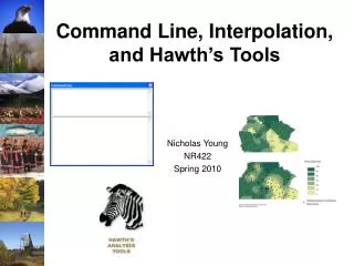
Command Line, Interpolation, and Hawth’s Tools. Nicholas Young NR422 Spring 2010. Outline. Command line What is command line? Learning from an Example Why use command line? Interpolation Definition Applications Types of interpolation Article examples Hawth’s Tools. Command Line.

E N D
Command Line, Interpolation, and Hawth’s Tools Nicholas Young NR422 Spring 2010
Outline • Command line • What is command line? • Learning from an Example • Why use command line? • Interpolation • Definition • Applications • Types of interpolation • Article examples • Hawth’s Tools
Command Line What is Command Line? • A way to interact with the or program by typing commands to perform certain tasks ?
Command Line • Location
The Interface Command Line Message section
Command Line • An Example: • Enter a tool name (may be different from Toolbox label)
Command Line Components • <> = Required parameter • {} = Optional parameter
Command Line Parameters Ex: Tool_name <in_raster> <other_parameters> <out_raster> • Parameter names for all input datasets are prefixed with "in_" and output datasets are prefixed with "out_". • The input dataset is usually the first parameter and the output dataset is usually the last required parameter. Other required parameters are placed between the input and output datasets.
Command Line Keywords Ex: {DEGREE | PERCENT_RISE} • Parameter with a fixed set of words allowed. • Keywords are always displayed in upper case • The "|“ means "or"
Command Line Colors of the Command Line Blue: Executed command line Black: Normal informational message Red: Error--Results were not created. Green: Warning-- Results may not be what you expect.
Command Line • Why use command line? • Not for all GIS users • But for Advanced and frequent geoprocessers, command line increases flexibility and speed of processing • Opening and filling out a tool's dialog is time-consuming. Typing commands is quicker and easier than using the tool dialog.
Command Line • Why use Command Line? • Execute multiple commands (string tasks)
Command Line • Why use Command Line • Recall commands previously executed changing to change its parameters if necessary and re-execute the command
Command Line • Why use Command Line • Save the commands you've typed to a text file and reload it later (simple scripting) • Similar to model builder (just not as colorful)
Why use Command Line? • Batch processing
Interpolation • Process of “intelligent guesswork” (Longley et al., 2005) • Attempts to make a reasonable estimate of the value of a field at places where the field has not actually been measured • Tobler’s Law http://webhelp.esri.com/arcgisdesktop/9.2/index.cfm?TopicName=Understanding_interpolation_analysis
Points to Raster http://webhelp.esri.com/arcgisdesktop/9.2/index.cfm?TopicName=Understanding_interpolation_analysis
Many Applications • Estimating rainfall, temp, etc. at locations with no direct measurements • DEMs • Contouring
Common Methods • Inverse Distance Weighting (IDW) • Spline • Trend • Kriging
Inverse Distance Weighting (IDW) • Estimates cell values by averaging the values of sample data points in the neighborhood of each processing cell • Uses weighted averages of observed values • Must have values between limits of measured values http://webhelp.esri.com/arcgisdesktop/9.2/index.cfm?TopicName=Understanding_interpolation_analysis
Spline • Estimates values using a mathematical function that minimizes overall surface curvature • Resulting surface must pass exactly through data points
Trend • Global polynomial interpolation that fits a smooth surface • Defined by a mathematical function (a polynomial) • Surface changes gradually and captures coarse-scale patterns in the data http://webhelp.esri.com/arcgisdesktop/9.2/index.cfm?TopicName=Understanding_interpolation_analysis
Kriging • Originally developed for mineral mapping • Predicts response as a linear function of the data and incorporates a weighting function between points that decays exponentially as distance between points increases • Kriging is a multistep process • Exploratory statistical analysis of the data • Variogram modeling • Producing the surface • Exploring a variance surface (optional)
Exploratory Analysis http://webhelp.esri.com/arcgisdesktop/9.2/index.cfm?TopicName=Understanding_interpolation_analysis
Semivariogram Semivariance Distance Semivariance = half the difference squared http://webhelp.esri.com/arcgisdesktop/9.2/index.cfm?TopicName=Understanding_interpolation_analysis0
Models • Circular • Spherical • Exponential • Gaussian • Linear http://webhelp.esri.com/arcgisdesktop/9.2/index.cfm?TopicName=Understanding_interpolation_analysis
Introduction • Geostatistical methods are valuable for analyzing spatial patterns of ecological systems • Visualization of prediction • Ecologists are unfamiliar with application of techniques • Urbanization creates distinct differences in community diversity J.S. Walker et al., 2008
Introduction • Use interpolation over habitat suitability models because of the lack of habitat suitability models for urban systems • Does not require a priori knowledge of habitat relationships J.S. Walker et al., 2008
Ordinary Kriging vs. Indicator Kriging • Does not assume data is normally distributed • Based on threshold values • Predicts the probability that a given location is above predetermined threshold • But prediction maps can not be generated • Data must conform to normality • Variogram is known • Prediction maps can be generated J.S. Walker et al., 2008
Data • Seasonal bird counts for 40 sites J.S. Walker et al., 2008
Data J.S. Walker et al., 2008
Data is Right Skewed J.S. Walker et al., 2008
Methods • Need to transform data for ordinary kriging • Used mean values for thresholds J.S. Walker et al., 2008
Semivariograms Nugget Range Autocorrelated Points not autocorrelated J.S. Walker et al., 2008
Model Comparison J.S. Walker et al., 2008
Conclusions • Both ordinary and indicator Kriging are viable tools for mapping species distributions • Both models were robust and had similar accuracy for all species • But indicator kriging does not require data transformation and there are few decision-making steps J.S. Walker et al., 2008
Hawth’s Tools • SpatialEcology.com • Developed by Hawthorne Beyer • Free to Download • Extension for ESRI's ArcGIS • “performs a number of spatial analyses and functions that cannot be conveniently accomplished with out-of-the-box ArcGIS”
Hawth’s Tools • Tools that automate mundane tasks • Tools that are designed to be part of an analysis workflow • Tools that target specific, ecology related analyses • Movement analysis, resource selection, predator prey interactions and trophic cascades
Hawth’s Tools • “[Dec 09] HawthsTools is now formally discontinued. The new software that replaces and improves upon Hawthstools is called the Geospatial Modelling Environment.”
New Hawth’s Tools?: Geospatial Modelling Environment • Designed to help to facilitate rigorous spatial analysis and modelling • uses the extraordinarily powerful open source software R as the statistical engine to drive some of the analysis tools
Geospatial Modelling Environment • Important update 1 March 2010: there is a newer version of the Statconn connector that is not recognized by the existing installer. I am writing a new installer that will greatly simplify the installation of GME and resolves the issue with 64-bit Windows and Windows 7. It should be ready shortly. I suggest you refrain from installing GME until I have this new installer ready. Thank you for your patience.