Spatial Prediction Methods in GIS: A Comprehensive Lecture Review
This lecture explores various spatial prediction methods used in GIS, reviewing key concepts from previous discussions. We categorize predictors into strata, global, local, and mixed approaches. Non-geostatistical methods are highlighted for their advantages and limitations. We delve into Kriging, stressing its importance as the Best Linear Unbiased Predictor (BLUP) that optimally predicts values based on spatial covariance. The practical application of Ordinary Kriging is discussed, along with regression derivations and essential steps to compute kriging weights and variances for effective geospatial analysis.

Spatial Prediction Methods in GIS: A Comprehensive Lecture Review
E N D
Presentation Transcript
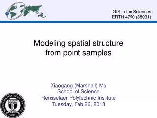
GIS in the Sciences ERTH 4750 (38031) Spatial prediction from point samples (2) Xiaogang (Marshall) Ma School of Science Rensselaer Polytechnic Institute Tuesday, Mar 19, 2013
Review of the last lecture • A taxonomy of spatial prediction methods • Strata: divide area to be mapped into “homogeneous” strata; predict within each stratum from all samples in that stratum • Globalpredictors: use all samples to predict at all points; also called regional predictors • Localpredictors: use only “nearby” samples to predict at each point • Mixed predictors: some of structure is explained by strata or globally, the residuals from this are explained locally
Review of the last lecture • Non-geostatistical prediction • Advantage: no model of spatial dependence is required; there is no need to compute or model variograms • Disadvantage: no theory behind them, only assumptions • We introduced: • Non-geostatistical stratified predictors • Non-geostatistical Local Predictors • Thiessenpolygons • Average within a radius • Distance-weighted average
Review of the last lecture • Kriging • A “Best Linear Unbiased Predictor” (BLUP) that satisfies a certain optimality criterion (so it's “best” with respect to the criterion) • Predicts at any point as the weighted average of the values at sampled points • Weights given to each sample point are optimal, given the spatial covariance structure as revealed by the variogram model (in this sense it is “best”) • The kriging variance at each point is automatically generated as part of the process of computing the weights.
How to use kriging in practice: • Sample • Calculate the experimental variogram • Authorized model(s) of the variogram • Apply the kriging system of equations at each point to be predicted • Calculate the variance of each prediction based on sample point locations • Display maps of both the predictions and their variances
Prediction with Ordinary Kriging (OK) • The most common form of kriging is usually called “Ordinary”. In OK, we model the value of variable at location as the sum of: • a regional mean and • a spatially-correlated random component . • The estimated value at a point is predicted as the weighted average of the values at all sample points : • The weights assigned to the sample points sum to 1:
Acknowledgements • This lecture is partly based on: • Rossiter, D.G., 2012. Spatial prediction from point samples (2). Lecture in distance course Applied Geostatistics. ITC, University of Twente
Contents • Regression derivation of the Ordinary Kriging (OK) system • Block Kriging (BK) • Universal Kriging (UK) • Regression derivation of the UK system
Deriving the kriging system • In the previous lecture we saw how to apply a model of local spatial dependence(i.e. a variogram model) to prediction by kriging. • To avoid information overload, we deferred discussing the kriging equations, and in particular in what sense kriging is an optimallocal predictor. • Note: It is not necessary to understand this topic completely in order to correctly apply kriging. The derivation is necessarily mathematical and in places requires knowledge of matrix algebra or differential calculus. Still, everyone who uses kriging should be exposed to this at least once.
Two approaches • There are two approaches to this derivation: • (1) Regression:As a special case of weighted least-squares prediction in the generalized linear model with orthogonal projections in linear algebra • (2) Minimization:Minimizing the kriging prediction variance with calculus • Approach (1) is mathematically more elegant and provides a clear link to well-established linear modeling theory, so we present it as the main derivation. • Approach (2) is an application of standard minimization methods from differential calculus; but is not so transparent, because of the use of LaGrange multipliers.
1 Regression derivation of the Ordinary Kriging equations • In this topic we show how to derive and solve the kriging equations. This provides a uniform framework for linear modeling (“regression”) and kriging. • This approach has four steps: • Model the spatial structure, e.g. the covariance function or semivariogram function; • Estimate the spatial mean; • Set up a kriging system to minimize the prediction variance; • Compute the kriging weights • The spatial mean centers the predictions; note that in Simple Kriging (SK, see below), the mean is known somehow, and this step is not necessary. • Step 1 has been discussed in a previous topic.
This topic requires a knowledge of matrix algebra and some familiarity with general linear models (e.g. weighted least-squares).
Step 2: estimate the spatial mean • The spatial mean of the variable to be predicted, over the study area , with area is: • In practice this is discretizedby summing over some fine grid: • where is the value of the variable at grid location . • But in general we do not have measurements at all locations! That's what we want to find out. So this equation can't be applied. We need to estimate the spatial mean from sparse observations (i.e. our sample points)
The spatial mean is not the average! • Problem: because of spatial autocorrelation, it is not correct simply to averagethe observations to obtain the mean. • If there is any spatial dependence, in general: Spatial mean Averageof the observations
The spatial mean • This is solved by weighted least squares, taking into account spatial correlation: • : a column vector of 1's; so : a row vector of 1's • In Universal Kriging (see below) this will be generalized to a design matrix ; here just a vector of 1's to estimate the mean • : the covariance matrix () among known points; • Note that so all diagonals are 1. • : the column vector of the known data values • This is a special case of Generalized Least Squares (GLS).
Breaking this down . . . • Two quadratic forms; both are and so end up as scalars; multiply two scalars to get the spatial mean: • Note: Let quadratic form in subsequent formulas. • If there is no spatial correlation, reduces to : all diagonals are 1, all off-diagonals are 0, the inverse , and this reduces to Ordinary Least Squares (OLS) estimation. • In this case (design matrix ), the OLS estimation of the spatial mean becomes the arithmetic average: the first quadratic term is and the second ; their product is
Spatial mean computed with semivariances • Recall: the semivarianceis the deviation of the covariance at some separation from the total variance: i.e. • But is constant (1) in the covariance functions; further, both quadratic forms include the matrix, so using its negative (plus a constant term), e.g. , does not change the solution. • In fact, we can replace by its difference from an arbitrary scalar (element-wise): • So semivariancesmay be used rather than covariancesin the formula for the spatial mean.
Step 3: Kriging prediction • Once we know the spatial mean, a kriging system can be set up without any additional constraints. • The special property of this system is that it is BLUP: “Best Linear Unbiased Predictor”, given the modeled covariance structure.
Formula for kriging prediction variance • By definition, the kriging prediction variance is: • the predicted value • : the (unknown) true value • For any weighted average, with weights , this is: • Kriging selects the weightsto minimize this expression.
Continued . . . • To make the division of weights clear, define two vectors of length : • where the first elements relate to the observation points and the last element to the prediction point. Then • The key point here is that the variance-covariance matrix is broken down into submatrices: for the covariance between sample points, for the covariance of each sample point with the prediction point, and for the variance at a point (the nugget).
Formula for kriging prediction • is the prediction at the prediction point • is the spatial mean computed in the previous step • is a column vector of the covariance between each sample point and the point to be predicted • the covariance matrix ( ) among known points • : the column vector of the known data values • : a column vector of 's, so that is a column vector of the means, and is a column vector of the residuals from the spatial mean
Breaking this down… • Note that the spatial mean is subtracted from each data value; so the right summand is the deviation from the spatial mean at the prediction point. • The spatial mean is added back in the left summand. • If there is no spatial dependence, and the prediction is just the spatial mean (which would then just be the average).
Step 4: Kriging weights • The OK prediction equation just derived does not explicitly give the weight to each observation; the kriging system can be used directly without computing these. • But we would often like to know the weights, to see the relative importance of each observation; also it may be more efficient to compute these and then the prediction as the weighted average. • Recall: the vector of kriging weights, is what to multiply each observation by in the weighted sum (prediction). • We get this by collecting all the terms that multiply the observed values in the OK prediction equation:
Kriging variance without weights • Above the prediction variance was computed for any set of weights; now we've selected weights to minimize the variance. Then the variance can be expressed without explicitly showing the weights. • We do this by substituting the expression for weights (previous step) into the expression for prediction variance (Step 3), to obtain: where: • is the nugget covariance (at separation 0) • Note: For block kriging, replace with , the average within-block variance (which will in general be smaller than the at-point variance); replace and with block-to-block covariances(see topic “Block Kriging”).
Kriging variance in terms of semivariances • Because of the relation (the semivarianceis the deviation of the covariance at some separation from the total variance): the kriging variance can also be expressed as: where: • is the matrix of semivariances between sample points • is the vector of semivariances between sample points and the point to be predicted • Note the change of sign, and that is now implicit.
2 Block Kriging (BK) • Often we want to predict average values of some target variable in blocks of some defined size, not at points. • Example: average woody biomass in a forest block of 40ha, if this is a minimum management unit, e.g. we will decide to harvest or not the whole block. We don't care about any finer-scale information, we wouldn’t use it if we had it. • Block kriging (BK) is quite similar in form to OK, but the kriging variances are lower, because the within-block variability is removed.
There is only one new idea in this section: by predicting an average over some block larger than the support, we reduce the kriging variance. • Most of this section shows how this is expressed mathematically. • The practical implication is shown in the comparative figures at the end of the section.
Block Ordinary Kriging (BK) • Estimate at blocks of a defined size, with unknown mean (which must also be estimated) and no trend • Each blockis estimated as the weighted average of the values at all sample points: • As with OK, the weights sum to 1, so that the estimator is unbiased, as for OK
The Block Kriging system • The same derivation as for the OK system produces these equations: • The semivariances are now between sample points and the blockto be predicted • The semivariance with a block is written as , the overline indicating an average • The left-hand side (semivariances between sample points) is the same as in OK
Solution Now we can estimate at the block, using the weights: The kriging variance for the block is given by: Note that the variance is reduced by the within-block variance.
The semivariancesin the above formulation are not just a function of separation, because they are not between points. Instead, they are between sample points and prediction blocks. This is illustrated in the following figure (left side). • In addition, the variance at the prediction location is now not at a point, but rather at a block. So some of the kriging variance must be accounted for within that block, i.e. the variance that is due to short-range variability at distances shorter than the block size. This is illustrated in the following figure (right side). • We will then discuss in detail how to compute these two.
Computing the semivariance between a point and a block • The complication here, compared to OK, is that the semivariances in the matrix are between sample points and the entire block to be predicted: • So there is not a single distance that can be substituted into the variogram model. We have to integrate over the block: • where is the area of the block, and is a point within the block. • As written all points in the block (conceptually, an infinite number!) would be used; In practice, this is done by discretization of the block into a set of points.
Computing the within-block variances • This is the factor by which the estimation variance is reduced: • As the block size approaches zero, the double integral also approaches zero; in fact this is the limit. This shows that OK is a special case of BK. • In practice, this is also calculated by discretizingthe block into points: • where of course ; the weights are set by their position within the unit block.
Visualizing the effect of block size • The following graphs show the changing predictionsand their variancesas the block size is increased. This is from the Meuse soil pollution study; target variable is log10(Cd). • Each graph uses one scale, to allow direct comparison.
Predictions: OK, BK10 BK40, BK160
Variances: OK, BK10 There is a very large reduction in variance with BK; increasing the block size reduces this still more but not as dramatically. BK40, BK160
3 Universal Kriging (UK) • This is a mixed predictor which includes a global trend as a function of the geographic coordinates in the kriging system, as well as local spatial dependence. • Example: The depth to the top of a given sedimentary layer may have a regional trend, expressed by geologists as the dip (angle) and strike (azimuth). However, the layer may also be locally thicker or thinner, or deformed, with spatial covariance in this local structure. • UK is recommended when there is evidence of first-order non-stationarity, i.e. the expected value varies across the map, but there is still second-order stationarityof the residuals from this trend. • Note: The “global” trend can also be fitted locally, within some user-defined radius, so that this interpolator can range from local (immediate neighborhood) to global (whole area), according to the analyst’s evidence on spatial structure.
An abstract view of UK/KED/RK • The realization of variable at spatial location can be considered as the result of three distinct processes: • a deterministiccomponent; e.g., a regional trend, or the effect of some forcing variable; • a spatially-correlatedstochastic process; • pure noise, not spatially-correlated, not deterministic
Relation of this formulation to trends and OK • OK: • i.e., the deterministic part is just a single expected value , the overall level of the target variable, with no spatial structure • The noise term is the nugget variance • Trend surface: • i.e., a deterministic trend (modeled from the coordinates) and noise • The noise term is the lack of fit
Prediction with UK • In UK, we model the value of variable at location as the sum of: • a regional non-stationary trend and • a local spatially-correlated random component ; the residuals from the regional trend • Note that the random component is now expected to be first-order stationary, because non-stationarity is all due to the trend • Here is not a constant as in OK, but instead is a function of position, i.e. the global trend.
Base functions • The trend is modeled as a linear combination of known base functionsand unknown constants (these are the parametersof the base functions):
Predictions at points • In UK, a point is predicted as in OK: • But, the weights for each sample point take into account both the global trend and local effects. • We need to set the UK system up to include both of these.
Computing the experimental semivariogram for UK • The semivariances are based on the residuals, not the original data, because the random field part of the spatial structure applies only afterany trend has been removed. • How to obtain? • Calculate the best-fit surface, with the same base functions to be used in UK; • Subtractthe trend surface at the data points from the data value to get residuals; • Compute the variogramof the residuals. • Note: Some programs, e.g. gstat, will do these all in one step.
Characteristics of the residual variogram • If there is a strong trend, the variogram model parametersfor the residuals will be very different from the original variogram model, since the global trend has taken out some of the variation, i.e. that due to the long-range structure. • The usual case is: • lower sill(less total variability) • shorter range(long-range structure removed)
Example original vs. residual variogram The trend surface removed much of the total variability, thereby lowering the total sill. In the variogram of residuals (in green color), the long-range variability (due to the trend) is removed, hence the shorter range of residuals.
Universal Kriging: Local vs. Global trends • As with OK, UK can be used in two ways: • Globally: using all sample points when predicting each point • Locally, or in patches: restricting the sample points used for prediction to some search radius (or sometimes number of neighbors) around the point to be predicted • We now discuss the properties of each
UK over the region • Using allsample points when predicting each point: • Appropriate if there is a regional trend across the entire study area • Agrees with the global computation of the residual variogram • This gives the same results as Regression Kriging on the coordinates