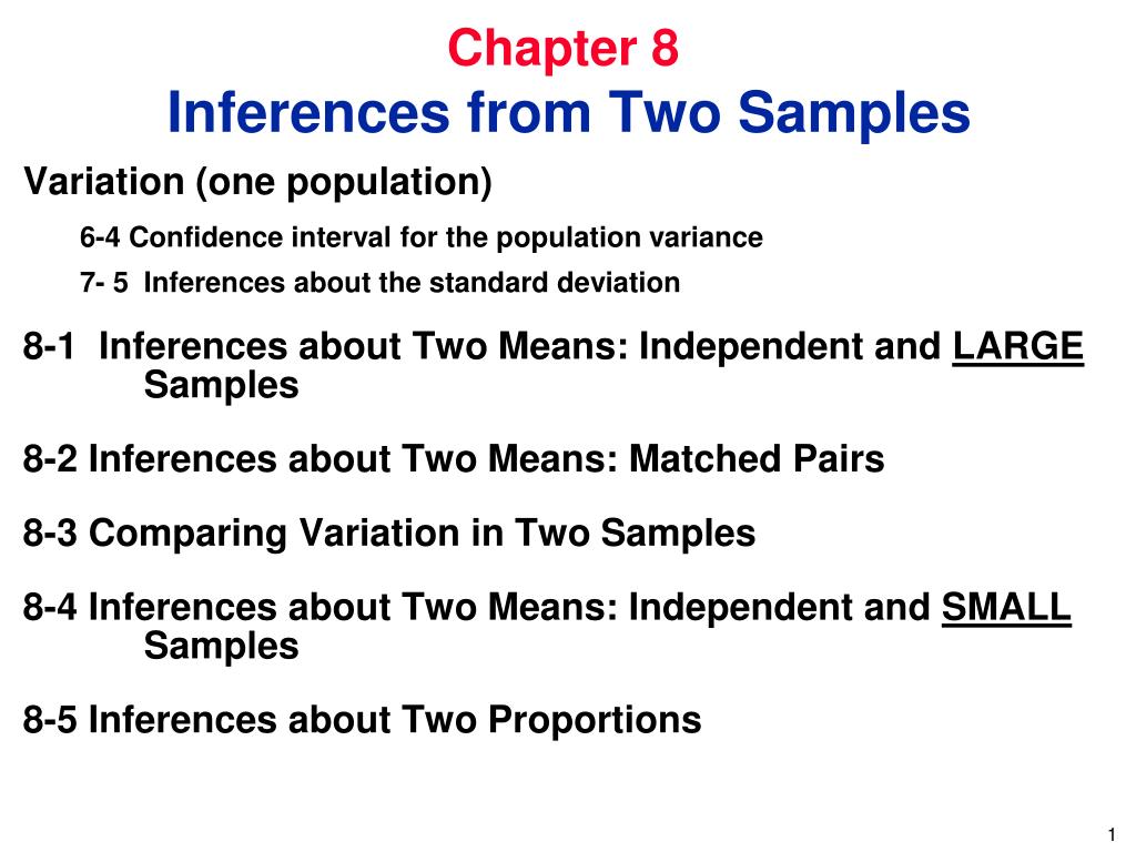
Chapter 8 Inferences from Two Samples

Variation (one population) 6-4 Confidence interval for the population variance 7- 5 Inferences about the standard deviation 8-1 Inferences about Two Means: Independent and LARGE Samples 8-2 Inferences about Two Means: Matched Pairs 8-3 Comparing Variation in Two Samples 8-4 Inferences about Two Means: Independent and SMALL Samples 8-5 Inferences about Two Proportions Chapter 8 Inferences from Two Samples

There are many important and meaningful situations in which it becomes necessary to compare two sets of sample data. Overview

6-4 Confidence interval for the population variance 7-5 Inferences about the standard deviation 8-3 Comparing Variation in Two Samples 6-4, 7-5, 8-3Estimation and Inferences Variation

6-4 Confidence interval for the population variance 7-5 Inferences about the standard deviation 8-3 Comparing Variation in Two Samples Estimation and Inferences Variation

1. The sample is a random sample. 2. The population must have normally distributed values (even if the sample is large). Assumptions

where n = sample size s 2= sample variance 2= population variance Chi-Square Distribution (n - 1) s 2 X 2= 2

Web Site Degrees of freedom (df ) = n - 1 X2 Critical Values found in theChi-Square Table

1. The chi-square distribution is not symmetric, unlike the normal and Student t distributions. As the number of degrees of freedom increases, the distribution becomes more symmetric. (continued) Properties of the Distribution of the Chi-Square Statistic df = 10 Not symmetric df = 20 x2 0 All values are nonnegative 5 10 20 25 30 35 40 45 15 0 Chi-Square Distribution for df = 10 and df = 20 Chi-Square Distribution

All values of X2 are nonnegative, and the distribution is not symmetric. There is a different distribution for each number of degrees of freedom. The critical values are found in the Chi-Square Table using n-1 degrees of freedom. Properties of Chi-Square Distribution

Chi-Square (x2) Distribution Area to the Right of the Critical Value Degrees of freedom 0.005 0.10 0.025 0.05 0.10 0.995 0.99 0.975 0.95 0.90 1 2 3 4 5 6 7 8 9 10 11 12 13 14 15 16 17 18 19 20 21 22 23 24 25 26 27 28 29 30 40 50 60 70 80 90 100 7.879 10.597 12.838 14.860 16.750 18.548 20.278 21.955 23.589 25.188 26.757 28.299 29.819 31.319 32.801 34.267 35.718 37.156 38.582 39.997 41.401 42.796 44.181 45.559 46.928 48.290 49.645 50.993 52.336 53.672 66.766 79.490 91.952 104.215 116.321 128.299 140.169 5.024 7.378 9.348 11.143 12.833 14.449 16.013 17.535 19.023 20.483 21.920 23.337 24.736 26.119 27.488 28.845 30.191 31.526 32.852 34.170 35.479 36.781 38.076 39.364 40.646 41.923 43.194 44.461 45.722 46.979 59.342 71.420 83.298 95.023 106.629 118.136 129.561 6.635 9.210 11.345 13.277 15.086 16.812 18.475 20.090 21.666 23.209 24.725 26.217 27.688 29.141 30.578 32.000 33.409 34.805 36.191 37.566 38.932 40.289 41.638 42.980 44.314 45.642 46.963 48.278 49.588 50.892 63.691 76.154 88.379 100.425 112.329 124.116 135.807 _ 0.020 0.115 0.297 0.554 0.872 1.239 1.646 2.088 2.558 3.053 3.571 4.107 4.660 5.229 5.812 6.408 7.015 7.633 8.260 8.897 9.542 10.196 10.856 11.524 12.198 12.879 13.565 14.257 14.954 22.164 29.707 37.485 45.442 53.540 61.754 70.065 3.841 5.991 7.815 9.488 11.071 12.592 14.067 15.507 16.919 18.307 19.675 21.026 22.362 23.685 24.996 26.296 27.587 28.869 30.144 31.410 32.671 33.924 35.172 36.415 37.652 38.885 40.113 41.337 42.557 43.773 55.758 67.505 79.082 90.531 101.879 113.145 124.342 _ 0.010 0.072 0.207 0.412 0.676 0.989 1.344 1.735 2.156 2.603 3.074 3.565 4.075 4.601 5.142 5.697 6.265 6.844 7.434 8.034 8.643 9.260 9.886 10.520 11.160 11.808 12.461 13.121 13.787 20.707 27.991 35.534 43.275 51.172 59.196 67.328 2.706 4.605 6.251 7.779 9.236 10.645 12.017 13.362 14.684 15.987 17.275 18.549 19.812 21.064 22.307 23.542 24.769 25.989 27.204 28.412 29.615 30.813 32.007 33.196 34.382 35.563 36.741 37.916 39.087 40.256 51.805 63.167 74.397 85.527 96.578 107.565 118.498 0.001 0.051 0.216 0.484 0.831 1.237 1.690 2.180 2.700 3.247 3.816 4.404 5.009 5.629 6.262 6.908 7.564 8.231 8.907 9.591 10.283 10.982 11.689 12.401 13.120 13.844 14.573 15.308 16.047 16.791 24.433 32.357 40.482 48.758 57.153 65.647 74.222 0.004 0.103 0.352 0.711 1.145 1.635 2.167 2.733 3.325 3.940 4.575 5.226 5.892 6.571 7.261 7.962 8.672 9.390 10.117 10.851 11.591 12.338 13.091 13.848 14.611 15.379 16.151 16.928 17.708 18.493 26.509 34.764 43.188 51.739 60.391 69.126 77.929 0.016 0.211 0.584 1.064 1.610 2.204 2.833 3.490 4.168 4.865 5.578 6.304 7.042 7.790 8.547 9.312 10.085 10.865 11.651 12.443 13.240 14.042 14.848 15.659 16.473 17.292 18.114 18.939 19.768 20.599 29.051 37.689 46.459 55.329 64.278 73.291 82.358

0.025 Critical Values: Table Areas to the right of each tail 0.975 0.025 0.025 0 2 XL2= 2.700 XR= 19.023 X 2 (df = 9)

The sample variance s is the best point estimate of the population variance 2 . Estimators of 2 2

2 (n - 1)s2 (n - 1)s2 X X 2 R Confidence Interval for the Population Variance 2 (n - 1)s2 (n - 1)s2 2  X X 2 L R Right-tail CV Left-tail CV Confidence Interval for the Population Standard Deviation   2 L

Example Find the confidence interval for IQ Scores of professional athletes ( assume population has a normal distribution) 1 – a = .90 n = 12 x = 104 s = 12

1. When using the original set of data to construct a confidence interval, round the confidence interval limits to one more decimal place than is used for the original set of data. 2. When the original set of data is unknown and only the summary statistics (n, s) are used, round the confidence interval limits to the same number of decimals places used for the sample standard deviation or variance. Roundoff Rule for Confidence Interval Estimates of  or 2

n = sample size s 2 = sample variance 2 = population variance (given in null hypothesis) (n - 1) s2 X 2 = 2 Chi-Square Distribution Test Statistic

Example:Aircraft altimeters have measuring errors with a standard deviation of 43.7 ft. With new production equipment, 81 altimeters measure errors with a standard deviation of 52.3 ft. Use the 0.05 significance level to test the claim that the new altimeters have a standard deviation different from the old value of 43.7 ft. 2= 0.025 Claim:  43.7 H0: = 43.7 H1:  43.7 = 0.05 0.975 n = 81 df = 80 Use Table 0.025 0.025 57.153 106.629

(n -1)s2 x2= =  114.586 (81 -1) (52.3)2  2 43.72 Reject H0 57.153 106.629 x2 = 114.586 The sample evidence supports the claim that the standard deviation is different from 43.7 ft.

(n -1)s2 x2= =  114.586 (81 -1) (52.3)2  2 43.72 Reject H0 57.153 106.629 x2 = 114.586 The new production method appears to be worse than the old method. The data supports that there is more variation in the error readings than before.

Table A-4 includes only selected values of  so specific P-values usually cannot be found Some calculators and computer programs will find exact P-values Don’t worry about finding p-values only know how to read them. P-Value Method

8-1 Inferences about Two Means:Independent and LARGE Samples

Two Samples: Independent The sample values selected from one population are not related or somehow paired with the sample values selected from the other population. If the values in one sample are related to the values in the other sample, the samples are dependent. Such samples are often referred to as matched pairs or paired samples. Definitions

1. The two samples are independent. 2. The two sample sizes are large. That is, n1> 30 and n2> 30. 3. Both samples are random samples. Assumptions

TI – 83 Procedure(s) for this Section • 2-SampZInt • 2-SampZTest • Note: Must know σ1 and σ2

Test Statistic for Two Means: Independent and Large Samples Hypothesis Tests (x1- x2) - (µ1 - µ2) Z*= 1. 2 2 2 + n2 n1

Null Hypothesis Ho : 1 = 2or Ho : 1 - 2= 0 Alternative Hypothesis H1 : 1≠2 H1 : 1>2 H1 : 1<2 Hypothesis Tests

Test Statistic for Two Means: Independent and Large Samples Hypothesis Tests Proceedure  and If and are not known, use s1 and s2 in their places. provided that both samples are large. Decision: Use the computed value of the test statistic z, the critical values and either the traditional or P-value method to draw your conclusion.

Men aged 25-34 Men aged 65-74 n 804 1657 x 176 164 σ 35 27 Sometimes is better to use a subscript that reflects something about each population instead of just 1 or 2 For example mo and my Weights of Men

Claim: average weights of older men is less that average weights of younger men. That is, o<y Ho : o = y H1 : o<y  = 0.01 Weights of Men Fail to reject H0 Reject H0 Z = - 2.33 1 -  = 0 or Z = 0

Test Statistic for Two Means: Independent and Large Samples Weights of Men (164 - 176) - 0 z*= 35 2 27 2 + 1657 804 = - 8.56

Claim: o<y Ho : o = y H1 : o<y  = 0.01 Weights of Men Fail to reject H0 Reject H0 Reject H0 Z = - 2.33 1 -  = 0 or Z = 0 -8.56

Claim: o<y Ho : o = y H1 : o<y  = 0.01 What about the p-value? P (z < -8.56) = ???? (very small) Weights of Men

Confidence Intervals (x1- x2) - E < (µ1 - µ2) < (x1- x2) + E 2 1 2 2 whereE = z + n2 n1

Confidence Intervals E = 2.575 (1.401) = 3.6 12 – 3.6 < (µy - µo) < 12 + 3.6 8.4 < (µy - µo) < 15.6 Can we use this confidence interval to test equality of means? Set up the hypothesis. Note: When calculating x1 – x2, always make it a positive value

8-2 Inferences about Two Means:Matched Pairs

1. The sample data consist of matched pairs. 2. The samples are random samples. 3. If the number of pairs of sample data is small (n  30), then the population of differences in the paired values must be approximately normally distributed. Assumptions

TI – 83 Procedure(s) for this Section • T-Test • T-Int • Note: (put differences in L1)

sd= standard deviation of the differences d for the paired sample data n = number of pairs of data. Notation for Matched Pairs µd= mean value of the differences d for the population of paired data d = mean value of the differences d for the paired sample data (equal to the mean of the x - y values)

Test Statistic for Matched Pairs of Sample Data d- µd t*= sd n where degrees of freedom = n - 1

Null Hypothesis Ho : d = 0 Alternative Hypothesis H1 : d≠0 H1 : d>0 H1 : d<0 Hypothesis Tests

Critical Values If n  30, critical values are found in Table A-3 (t-distribution). If n > 30, critical values are found in Table A- 2 (normal distribution).

degrees of freedom =n-1 Confidence Intervals d -E < µd < d + E sd where E =t/2 n

d = 11 sd = 20.24846 n = 10 t = -1.833 (found from Table A-3 with 10 degrees of freedom and 0.05 in two tails) Set up hypothesis, sketch and test the claim SAT Scores – HW #7

sd n Confidence Interval E =t/2 E = (2.262)( ) 20.24846 10 = 14.5

Confidence Interval -3.5 < µd< 25.5 • In the long run, 95% of such samples will lead to confidence intervals that actually do contain the true population mean of the differences. • Using the confidence interval to test the claim • Since the interval does contain 0, we FAIL TO REJECT H0, There is not sufficient evidence to support the claim that there is a difference between the scores for those student who took the preparatory course and those who didn’t.

Test Problem from this section will have data similar to

s = standard deviation of sample  = standard deviation of population s2 = variance of sample 2 = variance of population Measures of Variation

Assumptions 1. The two populations are independent of each other. 2. The two populations are each normally distributed. Comparing Variation in Two Samples

Chapter 8 Inferences from Two Samples

Télécharger la présentation

Plus de contenu associé