Download
1 / 74
740 likes | 785 Vues
Explore the principles and methodologies behind optic flow and motion detection in image sequences, including motion computation, optic flow, and practical applications in various fields. The text covers computation techniques, assumptions, solvability conditions, error sensitivity, iterative refinement, and the impact of motion scale. It also delves into the concepts of aperture problem, continuity constraints, and optimizing optic flow equations. Dive into small motion assumptions, edge gradients, texture regions, and iterative flow estimation strategies.

E N D
Optic Flow and Motion Detection Cmput 615 Martin Jagersand
Image motion • Somehow quantify the frame-to-frame differences in image sequences. • Image intensity difference. • Optic flow • 3-6 dim image motion computation
Motion is used to: • Attention: Detect and direct using eye and head motions • Control: Locomotion, manipulation, tools • Vision: Segment, depth, trajectory
Small camera re-orientation Note: Almost all pixels change!
MOVING CAMERAS ARE LIKE STEREO The change in spatial location between the two cameras (the “motion”) Locations of points on the object (the “structure”)
Classes of motion • Still camera, single moving object • Still camera, several moving objects • Moving camera, still background • Moving camera, moving objects
The optic flow field • Vector field over the image: [u,v] = f(x,y), u,v = Vel vector, x,y = Im pos • FOE, FOC Focus of Expansion, Contraction
Motion/Optic flow vectorsHow to compute? • Solve pixel correspondence problem • given a pixel in Im1, look for same pixels in Im2 • Possible assumptions • color constancy: a point in H looks the same in I • For grayscale images, this is brightness constancy • small motion: points do not move very far • This is called the optical flow problem
Optic/image flow Assume: • Image intensities from object points remain constant over time • Image displacement/motion small
Taylor expansion of intensity variation Keep linear terms • Use constancy assumption and rewrite: • Notice: Linear constraint, but no unique solution
Aperture problem f n f • Rewrite as dot product • Each pixel gives one equation in two unknowns: n*f = k • Min length solution: Can only detect vectors normal to gradient direction • The motion of a line cannot be recovered using only local information ò ó ò ó ð ñ î x î x @ I m @ I m @ I m à ît á r á = ; = I m @ t @ x @ y î y î y
The flow continuity constraint f f n n f f • Flows of nearby pixels or patches are (nearly) equal • Two equations, two unknowns: n1 * f = k1 n2 * f = k2 • Unique solution f exists, provided n1and n2not parallel
Sensitivity to error f f n n f f • n1and n2might be almost parallel • Tiny errors in estimates of k’s or n’s can lead to huge errors in the estimate of f
Using several points • Typically solve for motion in 2x2, 4x4 or larger image patches. • Over determined equation system: dIm = Mu • Can be solved in least squares sense using Matlab u = M\dIm • Can also be solved be solved using normal equations u = (MTM)-1*MTdIm
3-6D Optic flow • Generalize to many freedooms (DOFs)
All 6 freedoms X Y Rotation Scale Aspect Shear
Conditions for solvability • SSD Optimal (u, v) satisfies Optic Flow equation • When is this solvable? • ATA should be invertible • ATA entries should not be too small (noise) • ATA should be well-conditioned • Study eigenvalues: • l1/ l2 should not be too large (l1 = larger eigenvalue)
Edge • gradients very large or very small • large l1, small l2
Low texture region • gradients have small magnitude • small l1, small l2
High textured region • gradients are different, large magnitudes • large l1, large l2
Observation • This is a two image problem BUT • Can measure sensitivity by just looking at one of the images! • This tells us which pixels are easy to track, which are hard • very useful later on when we do feature tracking...
Errors in Optic flow computation • What are the potential causes of errors in this procedure? • Suppose ATA is easily invertible • Suppose there is not much noise in the image • When our assumptions are violated • Brightness constancy is not satisfied • The motion is not small • A point does not move like its neighbors • window size is too large • what is the ideal window size?
Iterative Refinement • Used in SSD/Lucas-Kanade tracking algorithm • Estimate velocity at each pixel by solving Lucas-Kanade equations • Warp H towards I using the estimated flow field - use image warping techniques • Repeat until convergence
Revisiting the small motion assumption • Is this motion small enough? • Probably not—it’s much larger than one pixel (2nd order terms dominate) • How might we solve this problem?
Coarse-to-fine optical flow estimation u=1.25 pixels u=2.5 pixels u=5 pixels u=10 pixels image H image I image H image I Gaussian pyramid of image H Gaussian pyramid of image I
Coarse-to-fine optical flow estimation warp & upsample run iterative L-K . . . image J image I image H image I Gaussian pyramid of image H Gaussian pyramid of image I run iterative L-K
HW accelerated computation of flow vectors • Norbert’s trick: Use an mpeg-card to speed up motion computation
Other applications: • Recursive depth recovery: Kostas and Jane • Motion control (we will cover) • Segmentation • Tracking
Lab: • Assignment1: • Purpose: • Intro to image capture and processing • Hands on optic flow experience • See www page for details. • Suggestions welcome!
Organizing Optic Flow Cmput 615 Martin Jagersand
Questions to think about Readings: Book chapter, Fleet et al. paper. Compare the methods in the paper and lecture • Any major differences? • How dense flow can be estimated (how many flow vectore/area unit)? • How dense in time do we need to sample?
Organizing different kinds of motion Two examples: • Greg Hager paper: Planar motion • Mike Black, et al: Attempt to find a low dimensional subspace for complex motion
Remember:The optic flow field • Vector field over the image: [u,v] = f(x,y), u,v = Vel vector, x,y = Im pos • FOE, FOC Focus of Expansion, Contraction
(Parenthesis)Euclidean world motion -> image Let us assume there is one rigid object moving with velocity T and w = d R / dt For a given point P on the object, we have p = f P/z The apparent velocity of the point is V = -T – w x P Therefore, we have v = dp/dt = f (z V – Vz P)/z2
Component wise: Motion due to translation: depends on depth Motion due to rotation: independent of depth
Remember last lecture: • Solving for the motion of a patch Over determined equation system: Imt = Mu • Can be solved in e.g. least squares sense using matlab u = M\Imt t t+1
3-6D Optic flow • Generalize to many freedooms (DOFs) Im = Mu
Know what type of motion(Greg Hager, Peter Belhumeur) u’i = A ui + d E.g. Planar Object => Affine motion model: It = g(pt, I0)
Mathematical Formulation • Define a “warped image” g • f(p,x) = x’ (warping function), p warp parameters • I(x,t) (image a location x at time t) • g(p,It) = (I(f(p,x1),t), I(f(p,x2),t), … I(f(p,xN),t))’ • Define the Jacobian of warping function • M(p,t) = • Model • I0 = g(pt, It ) (image I, variation model g, parameters p) • DI = M(pt, It) Dp (local linearization M) • Compute motion parameters • Dp = (MT M)-1MT DI where M = M(pt,It)
Planar 3D motion • From geometry we know that the correct plane-to-plane transform is • for a perspective camera the projective homography • for a linear camera (orthographic, weak-, para- perspective) the affine warp
Planar Texture Variability 1Affine Variability • Affine warp function • Corresponding image variability • Discretized for images
On The Structure of M Planar Object + linear (infinite) camera -> Affine motion model u’i = A ui + d X Y Rotation Scale Aspect Shear
Planar Texture Variability 2Projective Variability • Homography warp • Projective variability: • Where , and
Planar motion under perspective projection • Perspective plane-plane transforms defined by homographies
Planar-perspective motion 3 • In practice hard to compute 8 parameter model stably from one image, and impossible to find out-of plane variation • Estimate variability basis from several images: Computed Estimated
Another idea Black, Fleet) Organizing flow fields • Express flow field f in subspace basis m • Different “mixing” coefficients a correspond to different motions