Download

1 / 49
490 likes | 517 Vues
Stratocumulus. Adrian Lock. Over view. Stratocumulus climatology and recent changes in its representation in the Met Office climate model Summary of ‘important’ aspects of the boundary layer parametrization Other issues Cloud scheme complexity Resolution GCM dynamics and grid staggering.

E N D
Stratocumulus Adrian Lock
Overview • Stratocumulus climatology and recent changes in its representation in the Met Office climate model • Summary of ‘important’ aspects of the boundary layer parametrization • Other issues • Cloud scheme complexity • Resolution • GCM dynamics and grid staggering
Tropopause Inversion Cloud base Sub-tropics tropics Subsidence Inversion Entrainment Fq,T Fq,T Increasing SST Borrowed from Pier Siebesma
Stratocumulus climatology • Extensive cloud cover in the subtropics • Significant SW radiative impact (cooling the planet) • Errors lead to • SST errors in coupled climate models • surface temperature errors over land • Latest IPCC round includes an almost completely new Met Office model, HadGEM1
Climate model JJA total cloud amount HadGAM1(Released 2004) HadGAM1 - HadAM3(Released 1996) ISCCP HadGAM1 - ISCCP
Climate model improvement in low level cloud amount ISSCP HADAM3 (~1996) HadGAM1(~2004) • HadAM3 had excessive thick low cloud and too little thin • HadGAM1 very much better Thick (scale 0-20%) Intermediate (scale 0-40%)
GCM cross-section intercomparison (Siebesma et al 2004 and now GCSS) • GCMs, data from JJA 1998 • Cross-section from California to central Pacific • General underestimate of stratocumulus? • HadGAM1 not too bad • HadAM3 wouldn’t look too bad either HadGAM1 HadGAM1 total cloud cover California Central Pacific SSMI (all clouds) California HadGAM1 (low clouds) x x x x x x x x
Met Office GCM cloud fractionsEUROCS cross-section – 1998 JJA mean • HadGAM1 has more realistic boundary layer structure HadGAM1 (Released 2004) HadAM3 (Released 1996) Layer cloudfraction Convective cloud fraction ITCZ California ITCZ California
GPCI: SW radiation • More spread between models in radiation fluxes than in the clouds themselves • HadGAM1 has too much cloud in the Sc-Cu transition region HadGAM1 HadGAM1
LWP Diurnal cycle validation against satellite LWP kgm-2 • Wood et al (2002) analysed mean LWP diurnal cycle from satellite microwave measurements ( ) • Lock (2004) compared with HadGAM1 for the data from the EUROCS intercomparison (JJA in NE Pacific) HadGAM1: JJA mean LWP (kgm-2) x x Wood et al area x x x X EUROCS points
Validation against EPIC profiles • Comparison of HadGAM1 October mean profiles with mean profiles from EPIC for 16-21 October 2001 at (85W, 20S) • But HadGAM1 monthly mean LWP ~ 70gm-2 compared to the observed 150gm-2 HadGAM EPIC
Why the improvement from HadCM3 to HadGEM1? • Virtually everything is changed! • Doubled resolution (vertical and horizontal) • New dynamics • New Physics: • Microphysics • Cloud scheme (Smith + parametrized RHcrit) • Convection scheme (revised closure, triggering, CMT) • Radiation ~ the same?! • Plus new boundary layer scheme…
The new boundary layer parametrization in HadGEM1 • Old scheme (HadAM3) • Local Ri-dependent scheme • Kept for stable boundary layers in HadGEM1 • Non-local parametrization for unstable boundary layers • Specified (robust) profiles of turbulent diffusivities, for turbulence driven from the surface and/or cloud-top • Explicit BL top entrainment parametrization • Mass-flux convection scheme trigger based on boundary layer structure rather than local instability • BL mixes in subcloud layer, mass-flux in cloud layer • PBL scheme ~ a mixed layer model on a finite-difference grid
Mixed layer framework - motivation • Marine stratocumulus is often an equilibrium state arising from complicated interactions between many processes that are parametrized in GCMs • Need to replicate this balance within GCM parametrizations, often using schemes that currently operate independently • Simple conceptual framework: mixed layer model • turbulent mixing generally ensures that variables conserved under moist adiabatic ascent are close to uniform in the vertical. For example:
Observed profiles from stratocumulus Stevens et al (QJ,2003) Price (QJ, 1999)
Mixed layer model • Integrating over the boundary layer and assuming a discontinuous inversion gives the mixed layer model equations: where is the jump across the inversion and is the entrainment rate. • Mixed layer model is simple but effective • highlights the importance of entrainment
Entrainment efficiency (Stevens, 2002) • Cloud-top radiative cooling both cools the ML but also drives entrainment and so warms (and dries) it • Net effect of radiative cooling on ML evolution is therefore a strong function of the entrainment efficiency • Eg. for ‘minimal’ model: • Uncertain – parametrizations in the literature give widely different entrainment efficiencies (Stevens, 2002):
Entrainment efficiencies (Stevens, 2002) 0.5 0.4 • Differences in variability of entrainment efficiency as well as its magnitude • AL is noticeably weaker 0.9 0.8 0.7 0.7
Verification of entrainment parametrization against LES and observations LES Cloud free: = surface heated Smoke clouds: = radiatively cooled = surf heat + rad cool Water clouds: X = rad cool (no b.r.) + = rad cool + buoy rev = buoyancy reversal only Observations = Nicholls & Leighton,1986; Price, 1999; Stevens et al 2003 Actual entrainment rate (m/s) Parametrized entrainment rate (m/s)
Entrainmentparametrization in GCMs • Hard to parametrize on (coarse) GCM grids using traditional down-gradient diffusion because gradients at inversions are large and • K(Ri): local stability dependence is not relevant • K(z/zi): very sensitive to the definition of zi • K(TKE): accurate TKE evolution hard to resolve • Explicit parametrization requires a formulation for we • Uncertain • But you know what you are (or should be) getting
Numerical handling of inversions • All model processes (turbulence, radiation, LS advection) should be coupled to preserve mixed layer budgets • i.e., no spurious numerical transport across inversion(Stevens et al 1999, Lenderink and Holtslag 2000, Lock 2001, Grenier and Bretherton 2001, Chlond et al 2004) • Explicit BL top entrainment parametrization with flux-coupling • A subgrid inversion diagnosis takes tendencies from subsidence, radiation and turbulence and realistically distributes them between the mixed layer and the inversion grid-level – ‘inversion flux-coupling’ Free atmosphere ql profile (idealised mixed layer) x Entrainment x Real inversion (rises/falls) x GCM inversion grid-level (cools/warms) Subsidence x Mixed layer x
Diagnosis of subgrid mixed-layer model profile GCM cell-averages Subgrid profile • Identify ‘inversion grid-level’ • Extrapolate GCM profiles into the inversion grid-level • Assume a discontinous subgrid inversion • Calculate subgrid inversion height and strength X X X Inversion grid-level X Flux grid-levels X Parcel ascent vl = l( 1+rmqt )
Example calculation of grid-level entrainment fluxes (ignoring subsidence) X = GCM fluxes Radiative flux = mixed layer model fluxes • Subsidence fluxes across the inversion must be coupled similarly X X X Inversion grid-level X X X X X X X Flux grid-levels X Heat Fluxes
Impact of inversion treatment • Errors from not coupling fluxes amount to spurious additional entrainment • GCM: JJA mean liquid water path • SCM: Time-height contour plots of liquid water from simulations with subsidence > entrainment but ML budget (so cloud depth) stationary With inversion flux-coupling: With inversion flux-coupling Inversion height Impact of removing inversion flux-coupling: Without inversion flux-coupling
Equilibrium mixed layers – Stevens 2002 • Minimal model with entrainment efficiency of 0.5 • For this fixed entrainment efficiency, heading towards California (increasing divergence, reducing SST): • Strong response: zi decreases, wTsurf increases (contours) • Weaker response: LWP decreases, wqsurf decreases (grey-scales) • Minimal model not too far from reality Towards California
Mixed layer model sensitivity to entrainment efficiency • Minimal model with entrainment efficiency of 0.5 • Efficiency of 1: lower LWP, much reduced wTsurf Towards California
GCM cloud sensitivity to entrainment Std Met Office • Test GCM sensitivity to cloud-top entrainment • More active entrainment (either explicit or numerical) gives an equilibrium state with smaller surface heat fluxes and less stratocumulus (as in Stevens, 2002) • Removing inversion flux-coupling is more severe than doubling we 2 x we No flux coupling
Surface heat flux sensitivity to entrainment Standard Met Office • Expect spurious numerical entrainment to be • so increases as you approach the coast • Implies wT surf would reduce towards the coast • As it does if flux-coupling removed in Met Office GCM • As it does in other GCMs from EUROCS • Spurious or deliberate increase in parametrized entrainment efficiency? 2 x we No flux coupling
Entrainment efficiencies (Stevens, 2002) 0.5 0.4 • None of these proposed parametrizations show entrainment efficiency increasing ‘towards California’ 0.9 1.0 0.8 1.0 0.8 0.7 0.8 0.7
What about precipitation? • But AL is still a ‘weak’ entrainment parametrization • Is this being compensated for in HadGAM1 by a spuriously high drizzle rate? • Requires a drizzle climatology – satellite borne radar? HadGAM1 No obs!
Other issues • Cloud scheme • Prognostic vs diagnostic – does it matter? • Vertical resolution • Decoupling – structure within ‘mixed’ layers • New Dynamics
Other issues – cloud scheme complexity • Cloud-top height dependence on cloud scheme: HadGAM1 (Smith) PC2 (prognostic ql and CF)
Other issues – partial cloud cover Somewhere in between! CF~0.5 ? Near Hawaii CF~0.1 Convection scheme Near LA CF~1 BL scheme
AM2p12b ARPEGE Histograms of Cloud Cover JJA 1998 JJA 2003 all clouds low clouds (>700hPa) all clouds low clouds (>700hPa) CAM 3.0 number of events (%) GSM 0412 HadGAM RACMO2 Other issues – cloud scheme Cloud cover PDFs from GPCI • Medium cloud cover • Relatively low occurrence in HadGAM1 • Mixed layer model would break down • Possible cause of excessive cloud problems in Sc-Cu transition? Latitude HadGAM1: 0 Low cloud cover 1
Other issues • Cloud scheme • Vertical resolution • How much is sufficient? • Currently 38 levels ~280m at 1km ~ cloud thickness • Decoupling – structure within ‘mixed’ layers • New Dynamics
Lock (2001) Namibian Stratocumulus region31st March 2004 Model Level Striping in cloud fields not observed in albedo from GERB instrument (not shown)
Other issues • Cloud scheme • Vertical resolution • Decoupling – structure within ‘mixed’ layers • New Dynamics
Increasing the susceptibility to decoupling • EUROCS diurnal cycle of FIRE1 stratocumulus motivated changes to decoupling diagnosis (include subgrid cloudbase) • Operational testing (10 global forecast case studies) showed: • Reduced cloudiness, as expected • Significant improvement to tropical winds at 850hPa Change in total cloud cover Bias Control Revised scheme RMS speed error
Improved tropical winds hypothesis • Decoupling implies moister near surface implies reduced surface moisture fluxes in subtropical stratocumulus areas • Implies less moisture transported to tropics implies reduced tropical rainfall implies reduction in current model excessive tropical hydrological cycle implies beneficial reduction in trade wind strength • Implies mixed layer structure is important Change in total cloud cover Change in surface moisture flux
Other things • Cloud scheme • Vertical resolution • Decoupling – structure within ‘mixed’ layers • New dynamical formulation included: • Semi-implicit, semi-Lagrangian dynamics • Revised timestep (parallel calculation of ‘slow’ physics increments and BL diffusion coefficients) • Revised vertical grid staggering (better handling of normal modes and control of computational modes) • Showed a general improvement in low cloud • But no clean comparison (eg. with the same physics)
HadSM3 Cloud Response along GCSS Pacific Cross Section transect • Coupled atmosphere/slab-ocean models • Sc in HadSM4 (old dynamics) very different from HadGSM1 (new dynamics) • HadSM4 includes Lock et al (2000) scheme but not flux-coupling
Stratocumulus issues • Met Office model appears to have overcome the 1st order problem (it has stratocumulus-like clouds in some of the right places) but… • Entrainment • Still large spread in parametrizations (Stevens 2002) • Still large spread in LES (Duynkerke et al 2004 or Stevens et al 2005) • Is a special treatment of fluxes across inversions necessary in GCMs? • Need observed cloud-top height to validate NWP (eg. lidar or radar?) • Drizzle • Large term in mixed layer budget • How well is it represented in GCMs (lack of observed climatology)? • Role and parametrization of aerosols (cf land/sea split in NWP)? • Stabilising feedback on turbulent dynamics (Ackerman et al 2004)? • Mixed layer structure in subtropics is important for downwind deep convection in tropics • Beneficial impact from changes to decoupling • Testing revisions to non-local part of flux parametrization • How well-mixed are the wind profiles?
More parametrization issues • What level of cloud scheme complexity is necessary? • Smith scheme couples liquid water and cloud fraction too strongly • Is a prognostic scheme necessary for BL clouds? • Inhomogeneity – important for SW and drizzle • How to model partial cloud cover? • Massflux versus turbulent diffusion • Would unification help? • Communication would be easier (eg. Cu detraining into Sc) • Current massflux schemes seem incompatible with the top-down mixing predominant in stratocumulus • Debate is fuelled by a lack of understanding (limited case studies - need more extensive examination of parameter space) • If we knew (physically) how to parametrize BL clouds in general, wouldn’t the choice be made on numerical stability and accuracy?
Stratocumulus forecasting • Important for forecasting surface temperatures • Case study of widespread low cloud over Europe in December 2004 (eg. 12Z on the 10th) Low cloud fraction in global UM T+48 x x Budapest Thanks to Martin Kohler
Stratocumulus forecasting 12Z 10th December Surface mixed layer depth (m) • Boundary layer depth evolution mimics the observed • General underestimate of boundary layer depth by ~100m (< grid size) • General cold moist bias • Analysis tends to ‘decouple’ Day of December 2004
Spin-up of cloud in forecast models • Significant underestimate of cloud cover in the analysis followed by spin-up, at all horizontal resolutions
+ LW - CFMIP cloud feedback classes: Low positive class contributes most to uncertainty in sensitivity - SW +