Download
1 / 91
910 likes | 1.02k Vues
This dissertation defense explores the validity checking in first-order logic theories, focusing on quantifier-free formulas. The discussion covers the basics of first-order logic, theories, and validity concepts, analyzing decision procedures and applications. Notably, it delves into the limitations of existing tools like SVC and proposes new contributions and methodologies to enhance efficiency and performance in validity checking.

E N D
Checking Validity of Quantifier-Free Formulas in Combinations of First-Order Theories Clark W. Barrett Ph.D. Dissertation Defense Department of Computer Science Stanford University August 2001
The Problem: First-Order Logic • First-Order Logic is a mathematical system for making precise statements. • Statements in first-order logic are made up of the following pieces: • Variablesx, y • Constants0, John, • Functionsf (x ), x + y • Predicatesp (x ), x>y, x=y • Boolean connectives, , , • Quantifiers, • Example: “Every rectangle is a square” x. (Rectangle (x )Square(x))
The Problem: First-Order Theories • A first-order theory is a set of first-order statements about a related set of constants, functions, and predicates. • A theory of arithmetic might include the following statements about 0 and +: x. ( x+ 0 =x ) x,y. (x + y = y + x )
The Problem: Validity Valid Valid Valid Invalid • An expression is valid if every possible way of interpreting it results in a true statement. x =x p(x ) p(x ) x=y f (x ) =f (y ) f (x ) =f (y ) x=y • An expression is valid in atheory if every possible way of interpreting it in that theory results in a true statement. x 0 • An expression is valid in atheory if every possible way of interpreting it in that theory results in a true statement. x 0Invalid in the theory of real arithmetic • An expression is valid in atheory if every possible way of interpreting it in that theory results in a true statement. x 0Valid in positive real arithmetic
The Problem: Validity Checking • Suppose T is a first-order theory and is a first-order formula • We write T =as an abbreviation for “ is valid in T” • A classical result in Computer Science states that in general, the question of whether T = is undecidable. • It is impossible to write a program that can always figure out whether T = • However, given appropriate restrictions on T and , a program can automatically decide T = • We consider theories Tsuch that T = is decidable when is quantifier-free.
Motivation • Many interesting and practical problems can be solved by checking the validity of a formula in some theory. • As evidence of this claim, consider the following widely-used tools tools which include decision procedures for checking validity • PVS [Owre et al. ‘92] • STeP [Manna et al. ‘96, Bjørner ‘99] • ESC [Detlefs et al. ‘98] • Mona [Klarlund and Møller ‘98] • SVC [Barrett et al. ‘96]
The SVC Story • Roots in processor verification • [Burch and Dill ‘94] • [Jones et al. ‘95] • Internal use at Stanford • Symbolic simulation [Su et al. ‘98] • Software specification checking [Park et al. ‘98] • Infinite-state model checking [Das and Dill ‘01] • External use since public release in 1998 • Model Checking [Boppana et al. ‘99] • Theorem prover proof assistance [Heilmann ‘99] • Integration into programming languages [Day et al. ‘99] • Many others
The SVC Story • Despite its success, SVC has many limitations • Gaps in theoretical understanding • Outgrown its original software architecture • Unnecessarily slow performance in some cases • This thesis is the result of ongoing efforts to address these limitations. • New contributions to underlying theory • A flexible and efficient implementation • Techniques for faster and more robust performance
Outline • Validity Checking Overview • The Problem • Motivation • The SVC Story • Top-Level Algorithm • Methods for Combining Theories • Implementation • Adapting Techniques from Propositional Satisfiability • Contributions and Conclusions
true y > x x = y false y > x x = y true y > x x = y Top-Level Algorithm • Consider the following formula in the theory of arithmetic x > y y > x x = y • Step 1: Choose an atomic formula • Step 2: Consider two cases: • Replace the atomic formula with true • Replace the atomic formula is with false • Step 3: Simplify
true x = y true false Top-Level Algorithm • Consider the following formula in the theory of arithmetic x > y y > x x = y true y > x x = y false y > x x = y true y > x x = y x y y x x y This formula is unsatisfiable
Validity Checking Overview • A literalis an atomic formula or its negation • The validity checker is built on top of a core decision procedure for satisfiability in T of a set of literals. • The method for checking satisfiability will vary greatly depending on the theory in question • The most powerful technique for producing a satisfiability procedure is by combiningother satisfiability procedures
Outline • Validity Checking Overview • Methods for Combining Theories • The Problem • Shostak’s Method • The Nelson-Oppen Method • A Combined Method • Implementation • Adapting Techniques from Propositional Satisfiability • Contributions and Conclusions
The Problem • Consider the following theories: • Real linear arithmetic: +,-,0,1,…, • Arrays:s[i], update(s,i,v) • Uninterpreted functions and predicates: f (x ), p(x ),… • And the following set of literals in the combined theory: p (y) s= update (t, i, 0 ) x-y-z=0 z+s[i] = f (x-y) p (x- f (f (z) ) ) • Consider the following theories: • Real linear arithmetic: +,-,0,1,…, • Arrays:s[i], update(s,i,v) • Uninterpreted functions and predicates: f (x ), p(x ),… • And the following set of literals in the combined theory: p (y ) s = update (t, i, 0 ) x - y - z =0 z + s[i ] = f (x - y ) p (x - f (f (z ) ) ) • Consider the following theories: • Real linear arithmetic: +,-,0,1,…, • Arrays:s[i], update(s,i,v) • Uninterpreted functions and predicates: f (x ), p(x ),… • And the following set of literals in the combined theory: p (y ) s =update (t, i, 0 ) x - y - z =0 z + s[i ]= f (x - y ) p (x - f (f (z ) ) ) • Consider the following theories: • Real linear arithmetic: +,-,0,1,…, • Arrays:s[i], update(s,i,v) • Uninterpreted functions and predicates: f (x ), p(x ),… • And the following set of literals in the combined theory: p(y ) s = update (t, i, 0 ) x - y - z =0 z + s[i ] =f (x - y ) p(x -f (f (z ) ) ) • Consider the following theories: • Real linear arithmetic: +,-,0,1,…, • Arrays:s[i], update(s,i,v) • Uninterpreted functions and predicates: f (x ), p(x ),… • And the following set of literals in the combined theory: p (y ) s = update (t, i, 0 ) x - y - z =0 z + s[i ] = f (x - y ) p (x - f (f (z ) ) ) • Question: Given a method to decide satisfiability of literals in each theory, how do we decide the satisfiability of literals in the combined theory? • Two main approaches, each with advantages and disadvantages • Shostak [Shostak ‘84] • Nelson-Oppen [Nelson and Oppen ‘79]
Shostak’s Method • Has formed an ongoing strand of research • Originally published in 1984 [Shostak ‘84] • Several clarifying papers since then • [Cyrluk et al. ‘96] • [Ruess and Shankar ‘01] • Used in several automated deduction systems • PVS, STeP, SVC • Unfortunately, remains difficult to understand • Details are nonintuitive • Simple proof of correctness has been especially elusive • Contribution: A new presentation of a key subset of Shostak’s original algorithm.
Shostak’s Method: Canonizer • There are two main components in a Shostak satisfiability procedure: the canonizerand the solver. • The canonizer rewrites terms into a unique form • T=a = b canon (a ) =canon (b ) • Example: canonizer for linear arithmetic • Combines like terms • canon (x + x ) = 2x • Imposes an ordering on the variables • canon (y + x ) =x + y
Shostak’s Method: Solver • A set of equations Eis said to be in solved form if the left-hand side of each equation is a variable which appears only once in E in solved formnot in solved form x = y + z x = y + z w = z - a w = z + x v =3y + b 2v =3y+b • S means replace each left-hand side variable occurring in S with its corresponding right-hand side E (w + x + y + z ) =z - a +y +z + y + z
Shostak’s Method: Solver • The solvertransforms an equation into an equisatisfiable set of equations in solved form • If T=a b , then solve (a = b ) ={ false } • Otherwise: • solve (a = b ) =a set of equations E in solved form • T=(a = b x.E ) • x is a set of fresh variables appearing in E, but not in a or b. • Example: solver for real linear arithmetic • solve (x - y - z =0 ) = { x = y + z } • solve (x + 1 =x -1 ) = { false }
The Simplified Algorithm • Given a set of equations and disequations • Step 1: Use the solver to convert into an equisatisfiable set of equations E in solved form • Use a generalization of Gaussian elimination with back substitution
Choose matrix row E -x -3y +2z =-1 x -y -6z = 1 2x + y -10z= 3 The Simplified Algorithm • Given a set of equations and disequations • Step 1: Use the solver to convert into an equisatisfiable set of equations E in solved form • Select an equation from • Apply E as a substitution to • Solve to get E’ • Apply E’ as a substitution to E • Add E’ to E
Apply previous rows E -x -3y +2z =-1 x -y -6z = 1 2x + y -10z= 3 The Simplified Algorithm • Given a set of equations and disequations • Step 1: Use the solver to convert into an equisatisfiable set of equations E in solved form • Select an equation from • Apply E as a substitution to • Solve to get E’ • Apply E’ as a substitution to E • Add E’ to E Choose matrix row
Apply to previous rows E The Simplified Algorithm • Given a set of equations and disequations • Step 1: Use the solver to convert into an equisatisfiable set of equations E in solved form • Select an equation from • Apply E as a substitution to • Solve to get E’ • Apply E’ as a substitution to E • Add E’ to E Choose matrix row Apply previous rows Make pivot 1 x =-3y +2z +1 x -y -6z = 1 2x + y -10z= 3
E The Simplified Algorithm • Given a set of equations and disequations • Step 1: Use the solver to convert into an equisatisfiable set of equations E in solved form • Select an equation from • Apply E as a substitution to • Solve to get E’ • Apply E’ as a substitution to E • Add E’ to E Choose matrix row Apply previous rows Make pivot 1 Apply to previous rows x -y -6z = 1 2x + y -10z= 3 x =-3y +2z +1
E The Simplified Algorithm • Given a set of equations and disequations • Step 1: Use the solver to convert into an equisatisfiable set of equations E in solved form • Select an equation from • Apply E as a substitution to • Solve to get E’ • Apply E’ as a substitution to E • Add E’ to E Choose matrix row Apply previous rows Make pivot 1 Apply to previous rows x =-3y +2z +1 -3y +2z +1-y -6z =1 2x + y -10z= 3
E The Simplified Algorithm • Given a set of equations and disequations • Step 1: Use the solver to convert into an equisatisfiable set of equations E in solved form • Select an equation from • Apply E as a substitution to • Solve to get E’ • Apply E’ as a substitution to E • Add E’ to E Choose matrix row Apply previous rows Make pivot 1 Apply to previous rows x =-3y +2z +1 y =-z 2x + y -10z= 3
E The Simplified Algorithm • Given a set of equations and disequations • Step 1: Use the solver to convert into an equisatisfiable set of equations E in solved form • Select an equation from • Apply E as a substitution to • Solve to get E’ • Apply E’ as a substitution to E • Add E’ to E Choose matrix row Apply previous rows Make pivot 1 Apply to previous rows x =-3(-z)+2z +1 y =-z 2x + y -10z= 3
E The Simplified Algorithm • Given a set of equations and disequations • Step 1: Use the solver to convert into an equisatisfiable set of equations E in solved form • Select an equation from • Apply E as a substitution to • Solve to get E’ • Apply E’ as a substitution to E • Add E’ to E Choose matrix row Apply previous rows Make pivot 1 Apply to previous rows 2x + y -10z= 3 x =5z +1 y =-z
E The Simplified Algorithm • Given a set of equations and disequations • Step 1: Use the solver to convert into an equisatisfiable set of equations E in solved form • Select an equation from • Apply E as a substitution to • Solve to get E’ • Apply E’ as a substitution to E • Add E’ to E Choose matrix row Apply previous rows Make pivot 1 Apply to previous rows x =5z +1 y =-z 2(5z +1)+(-z )-10z=3
E The Simplified Algorithm • Given a set of equations and disequations • Step 1: Use the solver to convert into an equisatisfiable set of equations E in solved form • Select an equation from • Apply E as a substitution to • Solve to get E’ • Apply E’ as a substitution to E • Add E’ to E Choose matrix row Apply previous rows Make pivot 1 Apply to previous rows z =-1 x =5z +1 y =-z
E The Simplified Algorithm • Given a set of equations and disequations • Step 1: Use the solver to convert into an equisatisfiable set of equations E in solved form • Select an equation from • Apply E as a substitution to • Solve to get E’ • Apply E’ as a substitution to E • Add E’ to E Choose matrix row Apply previous rows Make pivot 1 Apply to previous rows z =-1 x =5(-1)+1 y =-(-1)
E The Simplified Algorithm • Given a set of equations and disequations • Step 1: Use the solver to convert into an equisatisfiable set of equations E in solved form • Select an equation from • Apply E as a substitution to • Solve to get E’ • Apply E’ as a substitution to E • Add E’ to E Choose matrix row Apply previous rows Make pivot 1 Apply to previous rows x =-4 y =1 z =-1
E 4242 2(1)-10(-4)6(-1-2(-4)) 2y -10x 6(z -2x) The Simplified Algorithm • Given a set of equations and disequations • Step 1: Use the solver to convert into an equisatisfiable set of equations E in solved form • Step 2: Use this set of equations together with the canonizer to check if any disequality is violated • For each a b • Check if canon (E (a ) ) =canon (E (b ) ) x =-4 y =1 z =-1
E 1- 4y x - z 4z +14z +1 1-4(-z)(5z +1)-z The Simplified Algorithm • Given a set of equations and disequations • Step 1: Use the solver to convert into an equisatisfiable set of equations E in solved form • Step 2: Use this set of equations together with the canonizer to check if any disequality is violated • For each a b • Check if canon (E (a ) ) =canon (E (b ) ) x =5z +1 y =-z
The Simplified Algorithm • Given a set of equations and disequations • Step 1: Use the solver to convert into an equisatisfiable set of equations E in solved form • Step 2: Use this set of equations together with the canonizer to check if any disequality is violated • For each a b • Check if canon (E (a ) ) =canon (E (b ) ) • Technical detail: • If there is more than one disequality, the theory must be convex
Shostak’s Method: Combining Theories • In what sense is this algorithm a method for combining theories? • Two Shostak theories T1 and T2 can often be combined to form a new Shostak theory T =T2T2 • Compose canonizers: canon=canon1ocanon2 • Often, solvers can also be combined • Treat terms from other theory as variables • Repeatedly apply solvers from each theory until resulting set of equations is in solved form
Shostak’s Method: Contributions • Shostak’s original algorithm is much more complicated because it includes a decision procedure for the theory of pure equality with uninterpreted functions • Why is the simplified version a contribution? • Can be applied directly to produce decision procedures, even combinations of decision procedures • Much easier to understand and prove correct • Provides intuition for understanding the original algorithm • Provides the foundation for a generalization of the original Shostak method based on a variation of Nelson-Oppen
Nelson-Oppen • Developed for the Stanford Pascal Verifier • [Nelson and Oppen ‘79] • [Nelson ‘80, Oppen ‘80] • Tinelli and Harandi discovered a new (simpler) proof and an important optimization • [Tinelli and Harandi ‘96] • Used in real systems • ESC • EHDM [von Henke et al. ‘88] • Vampyre [http://www-cad.eecs.berkeley.edu/~rupak/Vampyre]
Nelson-Oppen • Unlike Shostak, Nelson-Oppen does not impose a specific strategy on individual theories • Instead of a solver and canonizer, • Each theory provides a complete satisfiability procedure • Technical detail: Each theory must be stably infinite • There are two phases in the version of Nelson-Oppen presented by Tinelli and Harandi • Purification phase • Check phase
Nelson-Oppen: Purification Phase • Transform a set of literals in a combined theory to an equisatisfiable set of literals such that each literal is pure : • A pure literalcontains symbols from only a single theory • Consider again the following set of literals in a combined theory of arithmetic, arrays, and uninterpreted functions p(y ) s =update (t, i, 0 ) x - y - z =0 z + s[i ]=f(x - y ) p(x -f (f (z ) ) ) j =0
Nelson-Oppen: Purification Phase • Transform a set of literals in a combined theory to an equisatisfiable set of literals such that each literal is pure : • A pure literalcontains symbols from only a single theory • Consider again the following set of literals in a combined theory of arithmetic, arrays, and uninterpreted functions p(y ) s =update (t, i, j ) x - y - z = j z + s[i ]=f(x - y ) p(x -f (f (z ) ) ) j =0 j =0 k = s[i ]
Nelson-Oppen: Purification Phase • Transform a set of literals in a combined theory to an equisatisfiable set of literals such that each literal is pure : • A pure literalcontains symbols from only a single theory • Consider again the following set of literals in a combined theory of arithmetic, arrays, and uninterpreted functions p(y ) s =update (t, i, j ) x - y - z = j z + k=f(x - y ) p(x -f (f (z ) ) ) j =0 k = s[i ] j =0 k = s[i ] l = x - y m = z + k
Nelson-Oppen: Purification Phase • Transform a set of literals in a combined theory to an equisatisfiable set of literals such that each literal is pure : • A pure literalcontains symbols from only a single theory • Consider again the following set of literals in a combined theory of arithmetic, arrays, and uninterpreted functions p(y ) s =update (t, i, j ) l - z = j m=f(l ) p(x -f (f (z ) ) ) j =0 k = s[i ] l = x - y m = z + k
Nelson-Oppen: Purification Phase • Transform a set of literals in a combined theory to an equisatisfiable set of literals such that each literal is pure : • A pure literalcontains symbols from only a single theory • Consider again the following set of literals in a combined theory of arithmetic, arrays, and uninterpreted functions p(y ) s =update (t, i, j ) l - z = j m=f(l ) p(v ) j =0 k = s[i ] l = x - y m = z + k n =f (f (z ) ) ) v = x - n
Nelson-Oppen: Purification Phase • Transform a set of literals in a combined theory to an equisatisfiable set of literals such that each literal is pure : • A pure literalcontains symbols from only a single theory • Consider again the following set of literals in a combined theory of arithmetic, arrays, and uninterpreted functions p(y ) m=f(l ) p(v ) n =f (f (z ) ) ) s =update (t, i, j ) k = s[i ] l - z = j j =0 l = x - y m = z + k v = x - n
p(y ) m=f(l ) p(v ) n =f (f (z ) ) ) s =update (t, i, j ) k = s[i ] l - z = j j =0 l = x - y m = z + k v = x - n Nelson-Oppen: Check Phase Definitions • Shared variables are variables that appear in literals from more than one theory • Shared: l, z, j, y, m, k, v, n • Unshared: x, s, t, i • An arrangementof a set is a set of equalities that partitions the set into equivalence classes • Suppose S ={ a , b , c } • Some arrangements of S • { a b , a c , bc } { { a } , { b } , { c } } • { a = b , a c , bc } { { a , b } , { c } } • { a = b , a = c , b=c } { { a , b , c } }
Nelson-Oppen: Check Phase • Choose an arrangementAof the shared variables • For each theory, check if the set of literals pure in that theory together with the arrangement A is satisfiable • If an arrangement exists that is compatible with each set of literals, then the original set of literals is satisfiable in the combined theory Arithmetic l - z = j j =0 l = x - y m = z + k v = x - n Arrays s =update (t, i, j ) k = s[i ] Uninterpreted p(y ) m=f(l ) p(v ) n =f (f (z ) ) ) A (l, z, j, y, m, k, v, n )
Arithmetic x - y - z =0 z + s[i ]=f(x - y ) Arrays s =update (t, i, 0 ) Uninterpreted p(y ) p(x -f (f (z ) ) ) Nelson-Oppen: A Variation • Contribution : A Variation of Nelson-Oppen • The purification phase can be eliminated • Instead, simply partition the formulas according to the outer-most symbol p(y ) s =update (t, i, 0 ) x - y - z =0 z + s[i ]=f(x - y ) p(x -f (f (z ) ) )
Arithmetic x - y - z =0 z + s[i ]=f(x - y ) Arrays s =update (t, i, 0 ) Uninterpreted p(y ) p(x -f (f (z ) ) ) A (s[i ], x - y, f(x - y ), 0,y, z, f (f (z ) ), x -f (f (z ) ) ) Nelson-Oppen: A Variation • Contribution : A Variation of Nelson-Oppen • The purification phase can be eliminated • Instead, simply partition the formulas according to the outer-most symbol • Choose an arrangement A of the shared terms which appear in a term or formula belonging to another theory • For each theory, check if the set of literals assigned to that theory together with the arrangement is satisfiable • Terms with foreign symbols are treated as variables
Nelson-Oppen: A Variation • Contribution : A Variation of Nelson-Oppen • The purification phase can be eliminated • Instead, simply partition the formulas according to the outer-most symbol • Choose an arrangement A of the shared terms which appear in a term or formula belonging to another theory • For each theory, check if the set of literals assigned to that theory together with the arrangement is satisfiable • Terms with foreign symbols are treated as variables • Contributions of this variation • Fewer formulas given to each theory • Easier to implement • Easier to combine with Shostak
Combining Shostak and Nelson-Oppen • Theory requirements • Shostak requires convexity • Nelson-Oppen requires stable-infiniteness • Contribution : The following theorem relates the two Every convex first-order theory with no trivial models is stably-infinite • The proof is based on first-order compactness • Note: if a convex theory does admit trivial models, it can usually be modified to include the non-triviality axiom: x,y. x y