Feature Computation: Representing the Speech Signal
1.48k likes | 2.11k Vues
Feature Computation: Representing the Speech Signal. Bhiksha Raj and Rita Singh. A 30-minute crash course in signal processing. The Speech Signal: Sampling. The analog speech signal captures pressure variations in air that are produced by the speaker The same function as the ear

Feature Computation: Representing the Speech Signal
E N D
Presentation Transcript
Feature Computation: Representing the Speech Signal Bhiksha Raj and Rita Singh Signal Reperesentation
A 30-minute crash course in signal processing Signal Reperesentation
The Speech Signal: Sampling • The analog speech signal captures pressure variations in air that are produced by the speaker • The same function as the ear • The analog speech input signal from the microphone is sampled periodically at some fixed sampling rate Voltage Sampling points Time Analog speech signal Signal Reperesentation
The Speech Signal: Sampling • What remains after sampling is the value of the analog signal at discrete time points • This is the discrete-time signal Intensity Sampling points in time Time Signal Reperesentation
The Speech Signal: Sampling • The analog speech signal has many frequencies • The human ear can perceive frequencies in the range 50Hz-15kHz (more if you’re young) • The information about what was spoken is carried in all these frequencies • But most of it is in the 150Hz-5kHz range Signal Reperesentation
The Speech Signal: Sampling • A signal that is digitized at N samples/sec can represent frequencies up to N/2 Hz only • The Nyquist theorem • Ideally, one would sample the speech signal at a sufficiently high rate to retain all perceivable components in the signal • > 30kHz • For practical reasons, lower sampling rates are often used, however • Save bandwidth / storage • Speed up computation • A signal that is sampled at N samples per second must first be low-pass filtered at N/2 Hz to avoid distortions from “aliasing” • A topic we wont go into Signal Reperesentation
The Speech Signal: Sampling • Audio hardware typically supports several standard rates • E.g.: 8, 16, 11.025, or 44.1 KHz (n Hz = n samples/sec) • CD recording employs 44.1 KHz per channel – high enough to represent most signals most faithfully • Speech recognition typically uses 8KHz sampling rate for telephone speech and 16KHz for wideband speech • Telephone data is narrowband and has frequencies only up to 4 KHz • Good microphones provide a wideband speech signal • 16KHz sampling can represent audio frequencies up to 8 KHz • This is considered sufficient for speech recognition Signal Reperesentation
The Speech Signal: Digitization • Each sampled value is digitized (or quantized or encoded)into one of a set of fixed discrete levels • Each analog voltage value is mapped to the nearest discrete level • Since there are a fixed number of discrete levels, the mapped values can be represented by a number; e.g. 8-bit, 12-bit or 16-bit • Digitization can be linear (uniform) or non-linear (non-uniform) Signal Reperesentation
The Speech Signal: Linear Coding • Linear coding (aka pulse-code modulation or PCM) splits the input analog range into some number of uniformly spaced levels • The no. of discrete levels determines no. of bits needed to represent a quantized signal value; e.g.: • 4096 levels need a 12-bit representation • 65536 levels require 16-bit representation • In speech recognition, PCM data is typically represented using 16 bits Signal Reperesentation
The Speech Signal: Linear Coding • Example PCM quantizations into 16 and 64 levels: • Since an entire analog range is mapped to a single value, quantization leads to quantization error • Average error can be reduced by increasing the number of discrete levels 4-bit quantized values 6-bit quantized values Mapped to discrete value Analog range Analog Input Analog Input Signal Reperesentation
The Speech Signal: Non-Linear Coding • Converts non-uniform segments of the analog axis to uniform segments of the quantized axis • Spacing between adjacent segments on the analog axis is chosen based on the relative frequencies of sample values in that region • Sample regions of high frequency are more finely quantized quantized value Analog range Analog value Probability Min sample value max Signal Reperesentation
The Speech Signal: Non-Linear Coding • Thus, fewer discrete levels can be used, without significantly worsening average quantization error • High resolution coding around the most probable analog levels • Thus, most frequently encountered analog levels have lower quantization error • Lower resolution coding around low probability analog levels • Encodings with higher quantization error occur less frequently • A-law and m-law encoding schemes use only 256 levels (8-bit encodings) • Widely used in telephony • Can be converted to linear PCM values via standard tables • Speech systems usually deal only with 16-bit PCM, so 8-bit signals must first be converted as mentioned above Signal Reperesentation
Effect of Signal Quality • The quality of the final digitized signal depends critically on all the other components: • The microphone quality • Environmental quality – the microphone picks up not just the subject’s speech, but all other ambient noise • The electronics performing sampling and digitization • Poor quality electronics can severely degrade signal quality • E.g. Disk or memory bus activity can inject noise into the analog circuitry • Proper setting of the recording level • Too low a level underutilizes the available signal range, increasing susceptibility to noise • Too high a level can cause clipping • Suboptimal signal quality can affect recognition accuracy to the point of being completely useless Signal Reperesentation
Digression: Clipping in Speech Signals • Clipping and non-linear distortion are the most common and most easily fixed problems in audio recording • Simply reduce the signal gain (but AGC is not good) % % Clipped signal histogram Normal signal histogram Absolute sample value Absolute sample value Signal Reperesentation
First Step: Feature Extraction • Speech recognition is a type of pattern recognition problem • Q: Should the pattern matching be performed on the audio sample streams directly? If not, what? • A: Raw sample streams are not well suited for matching • A visual analogy: recognizing a letter inside a box • The input happens to be pixel-wise inverse of the template • But blind, pixel-wise comparison (i.e. on the raw data) shows maximum dis-similarity A A template input Signal Reperesentation
Feature Extraction (contd.) • Needed: identification of salient features in the images • E.g. edges, connected lines, shapes • These are commonly used features in image analysis • An edge detection algorithm generates the following for both images and now we get a perfect match • Our brain does this kind of image analysis automatically and we can instantly identify the input letter as being the same as the template Signal Reperesentation
Sound Characteristics are in Frequency Patterns • Figures below show energy at various frequencies in a signal as a function of time • Called a spectrogram • Different instances of a sound will have the same generic spectral structure • Features must capture this spectral structure M UW AA IY Signal Reperesentation
Computing “Features” • Features must be computed that capture the spectral characteristics of the signal • Important to capture only the salient spectral characteristics of the sounds • Without capturing speaker-specific or other incidental structure • The most commonly used feature is the Mel-frequency cepstrum • Compute the spectrogram of the signal • Derive a set of numbers that capture only the salient apsects of this spectrogram • Salient aspects computed according to the manner in which humans perceive sounds • What follows: A quick intro to signal processing • All necessary aspects Signal Reperesentation
Capturing the Spectrum: The discrete Fourier transform • Transform analysis: Decompose a sequence of numbers into a weighted sum of other time series • The component time series must be defined • For the Fourier Transform, these are complex exponentials • The analysis determines the weights of the component time series Signal Reperesentation
The complex exponential • The complex exponential is a complex sum of two sinusoids ejq = cosq + j sinq • The real part is a cosine function • The imaginary part is a sine function • A complex exponential time series is a complex sum of two time series ejwt = cos(wt) + j sin(wt) • Two complex exponentials of different frequencies are “orthogonal” to each other. i.e. Signal Reperesentation
The discrete Fourier transform + Ax + Bx = Cx Signal Reperesentation
The discrete Fourier transform + A x + B x = Cx DFT Signal Reperesentation
The discrete Fourier transform • The discrete Fourier transform decomposes the signal into the sum of a finite number of complex exponentials • As many exponentials as there are samples in the signal being analyzed • An aperiodic signal cannot be decomposed into a sum of a finite number of complex exponentials • Or into a sum of any countable set of periodic signals • The discrete Fourier transform actually assumes that the signal being analyzed is exactly one period of an infinitely long signal • In reality, it computes the Fourier spectrum of the infinitely long periodic signal, of which the analyzed data are one period Signal Reperesentation
The discrete Fourier transform • The discrete Fourier transform of the above signal actually computes the Fourier spectrum of the periodic signal shown below • Which extends from –infinity to +infinity • The period of this signal is 31 samples in this example Signal Reperesentation
The discrete Fourier transform • The kth point of a Fourier transform is computed as: • x[n] is the nth point in the analyzed data sequence • X[k] is the value of the kth point in its Fourier spectrum • M is the total number of points in the sequence • Note that the (M+k)th Fourier coefficient is identical to the kth Fourier coefficient Signal Reperesentation
The discrete Fourier transform • Discrete Fourier transform coefficients are generally complex • ejq has a real part cosq and an imaginary part sinq ejq = cosq + j sinq • As a result, every X[k] has the form X[k] = Xreal[k] + jXimaginary[k] • A magnitude spectrum represents only the magnitude of the Fourier coefficients Xmagnitude[k] = sqrt(Xreal[k]2 + Ximag[k]2) • A power spectrum is the square of the magnitude spectrum Xpower[k] = Xreal[k]2 + Ximag[k]2 • For speech recognition, we usually use the magnitude or power spectra Signal Reperesentation
The discrete Fourier transform • A discrete Fourier transform of an M-point sequence will only compute M unique frequency components • i.e. the DFT of an M point sequence will have M points • The M-point DFT represents frequencies in the continuous-time signal that was digitized to obtain the digital signal • The 0th point in the DFT represents 0Hz, or the DC component of the signal • The (M-1)th point in the DFT represents (M-1)/M times the sampling frequency • All DFT points are uniformly spaced on the frequency axis between 0 and the sampling frequency Signal Reperesentation
The discrete Fourier transform • A 50 point segment of a decaying sine wave sampled at 8000 Hz • The corresponding 50 point magnitude DFT. The 51st point (shown in red) is identical to the 1st point. Sample 50 is the 51st point It is identical to Sample 0 Sample 50 = 8000Hz Sample 0 = 0 Hz Signal Reperesentation
The discrete Fourier transform • The Fast Fourier Transform (FFT) is simply a fast algorithm to compute the DFT • It utilizes symmetry in the DFT computation to reduce the total number of arithmetic operations greatly • The time domain signal can be recovered from its DFT as: Signal Reperesentation
Windowing • The DFT of one period of the sinusoid shown in the figure computes the Fourier series of the entire sinusoid from –infinity to +infinity • The DFT of a real sinusoid has only one non zero frequency • The second peak in the figure also represents the same frequency as an effect of aliasing Signal Reperesentation
Windowing • The DFT of one period of the sinusoid shown in the figure computes the Fourier series of the entire sinusoid from –infinity to +infinity • The DFT of a real sinusoid has only one non zero frequency • The second peak in the figure also represents the same frequency as an effect of aliasing Signal Reperesentation
Windowing Magnitude spectrum • The DFT of one period of the sinusoid shown in the figure computes the Fourier series of the entire sinusoid from –infinity to +infinity • The DFT of a real sinusoid has only one non zero frequency • The second peak in the figure also represents the same frequency as an effect of aliasing Signal Reperesentation
Windowing • The DFT of any sequence computes the Fourier series for an infinite repetition of that sequence • The DFT of a partial segment of a sinusoid computes the Fourier series of an inifinite repetition of that segment, and not of the entire sinusoid • This will not give us the DFT of the sinusoid itself! Signal Reperesentation
Windowing • The DFT of any sequence computes the Fourier series for an infinite repetition of that sequence • The DFT of a partial segment of a sinusoid computes the Fourier series of an inifinite repetition of that segment, and not of the entire sinusoid • This will not give us the DFT of the sinusoid itself! Signal Reperesentation
Windowing Magnitude spectrum • The DFT of any sequence computes the Fourier series for an infinite repetition of that sequence • The DFT of a partial segment of a sinusoid computes the Fourier series of an inifinite repetition of that segment, and not of the entire sinusoid • This will not give us the DFT of the sinusoid itself! Signal Reperesentation
Windowing Magnitude spectrum of segment Magnitude spectrum of complete sine wave Signal Reperesentation
Windowing • The difference occurs due to two reasons: • The transform cannot know what the signal actually looks like outside the observed window • We must infer what happens outside the observed window from what happens inside • The implicit repetition of the observed signal introduces large discontinuities at the points of repetition • This distorts even our measurement of what happens at the boundaries of what has been reliably observed Signal Reperesentation
Windowing • The difference occurs due to two reasons: • The transform cannot know what the signal actually looks like outside the observed window • We must infer what happens outside the observed window from what happens inside • The implicit repetition of the observed signal introduces large discontinuities at the points of repetition • This distorts even our measurement of what happens at the boundaries of what has been reliably observed • The actual signal (whatever it is) is unlikely to have such discontinuities Signal Reperesentation
Windowing • While we can never know what the signal looks like outside the window, we can try to minimize the discontinuities at the boundaries • We do this by multiplying the signal with a window function • We call this procedure windowing • We refer to the resulting signal as a “windowed” signal • Windowing attempts to do the following: • Keep the windowed signal similar to the original in the central regions • Reduce or eliminate the discontinuities in the implicit periodic signal Signal Reperesentation
Windowing • While we can never know what the signal looks like outside the window, we can try to minimize the discontinuities at the boundaries • We do this by multiplying the signal with a window function • We call this procedure windowing • We refer to the resulting signal as a “windowed” signal • Windowing attempts to do the following: • Keep the windowed signal similar to the original in the central regions • Reduce or eliminate the discontinuities in the implicit periodic signal Signal Reperesentation
Windowing • While we can never know what the signal looks like outside the window, we can try to minimize the discontinuities at the boundaries • We do this by multiplying the signal with a window function • We call this procedure windowing • We refer to the resulting signal as a “windowed” signal • Windowing attempts to do the following: • Keep the windowed signal similar to the original in the central regions • Reduce or eliminate the discontinuities in the implicit periodic signal Signal Reperesentation
Windowing Magnitude spectrum • The DFT of the windowed signal does not have any artefacts introduced by discontinuities in the signal • Often it is also a more faithful reproduction of the DFT of the complete signal whose segment we have analyzed Signal Reperesentation
Windowing Magnitude spectrum of original segment Magnitude spectrum of windowed signal Magnitude spectrum of complete sine wave Signal Reperesentation
Windowing • Windowing is not a perfect solution • The original (unwindowed) segment is identical to the original (complete) signal within the segment • The windowed segment is often not identical to the complete signal anywhere • Several windowing functions have been proposed that strike different tradeoffs between the fidelity in the central regions and the smoothing at the boundaries Signal Reperesentation
Windowing • Cosine windows: • Window length is M • Index begins at 0 • Hamming: w[n] = 0.54 – 0.46 cos(2pn/M) • Hanning: w[n] = 0.5 – 0.5 cos(2pn/M) • Blackman: 0.42 – 0.5 cos(2pn/M) + 0.08 cos(4pn/M) Signal Reperesentation
Windowing • Geometric windows: • Rectangular (boxcar): • Triangular (Bartlett): • Trapezoid: Signal Reperesentation
Zero Padding • We can pad zeros to the end of a signal to make it a desired length • Useful if the FFT (or any other algorithm we use) requires signals of a specified length • E.g. Radix 2 FFTs require signals of length 2n i.e., some power of 2. We must zero pad the signal to increase its length to the appropriate number • The consequence of zero padding is to change the periodic signal whose Fourier spectrum is being computed by the DFT Signal Reperesentation
Zero Padding • We can pad zeros to the end of a signal to make it a desired length • Useful if the FFT (or any other algorithm we use) requires signals of a specified length • E.g. Radix 2 FFTs require signals of length 2n i.e., some power of 2. We must zero pad the signal to increase its length to the appropriate number • The consequence of zero padding is to change the periodic signal whose Fourier spectrum is being computed by the DFT Signal Reperesentation
Zero Padding Magnitude spectrum • The DFT of the zero padded signal is essentially the same as the DFT of the unpadded signal, with additional spectral samples inserted in between • It does not contain any additional information over the original DFT • It also does not contain less information Signal Reperesentation
Magnitude spectra Signal Reperesentation


![[Advanced] Speech & Audio Signal Processing](https://cdn2.slideserve.com/3915760/advanced-speech-audio-signal-processing-dt.jpg)