Speech and Audio Coding
Speech and Audio Coding. Heejune AHN Embedded Communications Laboratory Seoul National Univ. of Technology Fall 2013 Last updated 2013. 9. 31. Audio Coding. Audio signal classes speech signal : 300Hz - 3400Hz (< 4KHz) For telephone service, e.g. VoIP, mobile voice telephony


Speech and Audio Coding
E N D
Presentation Transcript
Speech and Audio Coding Heejune AHN Embedded Communications Laboratory Seoul National Univ. of Technology Fall 2013 Last updated 2013. 9. 31
Audio Coding • Audio signal classes • speech signal : 300Hz - 3400Hz (< 4KHz) • For telephone service, e.g. VoIP, mobile voice telephony • wide speech signal : 50 - 7000Hz • High quality voice telephony. e.g . Skype, W-AMR in 3.5/4 G • wideband audio signal : - 20KHz • Entertainment. E.g. CD, mp3, DVD, broadcasting, cinema movies • CD example • Sampling frequency : 44.1 KHz • 16-bits/ sample • two stereo channels • net bit-rate = 2 x 16 x 44.1 x 10 = 1.41 Mbits/sec. • real bit-rate = 1.41 x 49/16 Mbit/sec = 4.32 Mbit/sec. • for synchronization and error correction, 49 bits for every 16-bit audio sample.
Audio coding techniques • Speech coding • Sound generation model is well studied • Wave form coding (time-domain) • Linear PCM, Non-linear PCM, DPCM, ADPCM • Vocoder • Use speech specific speech production model • Analysis at encoders and Synthesis at decoders. • LP-Vocoder, RPE (regular pulse excited) Vocoder (GSM), Q-CELP (qualcomm code-excited Linear prediction) (CDMA), AMR (Adaptive Multi-Rate) (Algebric code excited LP, 3G, 4G) • Audio coding • No sound generation model yet. • Human auditory system and psychoacoustic perception • MPEG1L1, 2, 3, MPEG-2 AAC, Dolby AC-3
Speech Coding • Signals
Linear PCM • Linear • Uniform Quantizer, i.e., quantization levels are evenly spaced. • SNR = 6 * no of bits + C db • at least 6*12 db required for human intelligible • 16-bit samples provide plenty of dynamic range. • Application • In CD, File formats of WAV (MS), AIFF (Unix and Mac)
Nonlinear PCM • Nonlinear • Non-uniform quantization • Quantization step-size decreases logarithmically with signal level • Using that the human audio perception is logarithm-scale • Companding • Compress and Expand before Uniform quantization • u-law and A-law
Mu law • Provides 14-bit quality (dynamic range) with an 8-bit encoding • Compression factor 2:1. • au (Sun audio file format). • in North American & Japanese ISDN voice service
DPCM • Predictive Coding • Transmit the difference (rather than the sample). • Difference between 2 x-bit samples can be represented with significantly fewer than x-bits
Slope-overload problem in DPCM • Prediction differences x(n) are too large for the quantizer to handle. Encoder fails to track rapidly changing signals. • Especially near the Nyquist frequency.
ADPCM • Adaptive step size • a larger step-size for fast-varying (high-frequency) samples; a smaller step-size for slowly varying samples. • Step size parameter is not transmitted; Use previous sample values to estimate changes in the signal in the near future.
Speech Production Model • Lung • Glottis/vocal cord : 성대 (pulse) • Vocal track (filter) • Cavities (articulation) • Organ model: change the vocal track filter • 2 Modes • voiced sound: vocal cord is vibrating (quasi-periodic excitation) • Unvoiced sound : vocal cord is open (noise like model) glittis cavities Lung Vocal cord Vocal track Lips/tungs
Signal and System modeling • Voiced Speech Lambda = 4L c= 340m/s Formant Frequencies f1= 340/4*0.17 = 500 Hz f3 = 1500 Hz f5 = 2500 Hz Time varying Linear system Excitation generation Vocal track + Radiation effect Train of glottal pulse T = pitch frequency T
Unvoiced Speech • No tonic excitation, no formant frquencies
Linear Predictive Coding • LPC • A generalization of ADPCM • Linear prediction model • Prediction parameters : changes slowly relatively the data rate … synthesis decoder M/sec Analysis Encoder at N /sec at N /sec at N/sec
Speech analysis and synthesis • In every 5 to 40 m • Analysis • Extract pitch frequencies • Spectral analysis : Using multiple band-pass filers. • Synthesis • Based on mode, excitation signal generate into the vocal track filter.
LPC analyzer decoder coder S(n) Pitch Detector (period, gain) Voice/unvoiced ? LPC synthesizer
Psychoacoustic Principles • Psycho-acoustic • Human auditory perception property, similar to HVS in Video Coding • Average human does not hear all frequencies the same way. • Limitations of the human sensory system leads to facts that can be used to cut out unnecessary data in an audio signal. • Key Properties • Critical Band Property • Masking Property ‘ • Absolute Threshold of hearing • Auditory masking
CriticalBands • Human auditory • Limited and frequency dependant Resolution • 25 critical bands • Bands • 1 Bark (e.g. Band) = the width of one critical band • Critical band number (Bark) for a given frequency, z(f): • f < 500Hz => z(f) ≈ f/100 • f > 500Hz => z(f) ≈ 9 + 4 log2(f/1000)
Absolute threshold of hearing • Range: 20 Hz - 20 kHz, most sensitive at 2 kHz to 4 kHz. • Dynamic range (quietest to loudest is about 96 dB) • Normal voice range is about 500 Hz - 2 kHz.
Simultaneous Masking • Masking Effects • The presence of tones at certain frequencies makes us unable to perceive tones at other “nearby” frequencies • Humans cannot distinguish between tones within 100 Hz at low frequencies and 4 kHz at high frequencies.
Approximates a triangular function modeled by spreading function, SF (x) (db), where x has units of bark less sleep sleeper
Example • Hopefully we can built demo.
TemporalMasking • If we hear a loud sound, then it stops, it takes a little while until we can hear a soft tone nearby. • As much as 50 ms before and 200 ms after. • Example; • Play 1 kHz masking tone at 60 dB and 1.1 kHz test tone at 40dB.
MPEG-1Audio • MP3 • Mostly popular audio format at present. • denotes MPEG-1 Audio Level 3, not MPEG-3 (no such a thing in the world) • Part of MPEG-1 Standards • 1.2 Mbps for video + 0.3 Mbps for audio • Sampling frequency • 32, 44.1 and 48 kHz • One or two audio channels • Monophonic, Dual-monophonic, Stereo, Joint Stereo • Compression ratio from 2.7:1 to 42:1 • Uncompressed CD audio - 44,100 samples/sec * 16 bits/sample * 2 ch > 1.4 Mbps • 16 bit stereo sampled at 48 kHz is reduced to 256 kbps
MPEG-1AudioLevels • Level of Complexity • Layer 1 • DCT type filter with one frame and equal frequency spread per band. • Psychoacoustic model only uses frequency masking. • Layer 2 • Use three frames in filter (before, current, next, a total of 1152 samples). • This models a little bit of the temporal masking. • Layer 3 (Known as MP3) • Better critical band filter is used (non-equal frequencies) • Psychoacoustic model includes temporal masking effects, and takes into account stereo redundancy. • Huffman coder.
Subband Bank • 32 PCM samples yields 32 subband samples. • Each sub-band evenly spaced, not like critical bands’ width • For example, @48 kHz sampling rate, each sub-band is 750 Hz wide. • Frame • Samples out of each filter are grouped into blocks, called frames. • Blocks of 12 for Layer 1 (384 samples). • Blocks of 36 for Layers 2 and 3(1152 samples) @48 kHz, 32x12 represents 8ms of audio.
Psychoacousticanalysis • FFT gets detailed spectral information about the signal. • 512-point FFT for Layer 1, 1024-point for Layer 2 and 3 • Don’t be confused the subband filter input samples! • Tonal and NonTonal masker from each band • Determine the minimal masking threshold in each subband. (using global threshold and masking threshold) • Calculate the signal-to-mask ratio (SMR) in each subband, • This can be considered a quantization margin.
Segment the signal into 512 samples => 12 ms frames • @44.1kHz
Maskingexample • Suppose the levels of the first 16 of the 32 sub-bands are: • Band !1 !2 !3 !4 !5 !6 !7 !8 !9 !10 !11 !12 !13 !14 !15 !16! • Level !0 !8 !12 !10 !6 !2 !10 !60 !35 !20 !15 !2 !3 !5 !3 !1! (dB) • The level of the 8th band is 60 dB, the pre-computed masking model specifies a masking of 12 dB in the 7th band and 15 dB in the 9th. • The signal level in 7th band is 10 (< 12 dB), so ignore it. • The signal level in 9th band is 35 (< 15 dB), so send it. • Only the signals above the masking level needs to be sent.
Scaling • In order to use full range of quantizer • Encoder : divide signal by scale factor before quantization • Decoder : multiply by scale factor after quantization • Scale Factor • Largest signal quantized using 6-bit scale-factor. • The receiver needs to know the scale factor and quantisation levels used. • Information included along with the samples • The resulting overhead is very small compared with the compression gains.
Bit allocation and Quantization • Constraints • the target bit rate. 192 kbps target rate => 8 ms/frame @48KHz => ~1.5 kbits/frame. • Objective • Objective is to minimize noise-to-mask ratio (NMR) over all sub-bands, i.e., minimize quantization noise. • Mission • For each audio frame, bits must be distributed across the sub-bands from a predetermined number of bits defined by bit-allocation frames 12 data/ frame/band 1/scaling factor quantizer
A solution for bit allocation • More bits for low Mask Level (since noise is easily noticed) • Iterative process • For each sub-band, determine NMR = SNR – SMR • Allocate bits one at a time to the sub-band with the largest NMR. Recalculate NMR values.Iterate until all bits used.
Output Frame • Frame format • Framelen - frame length in bytes; • Bit-allocation: • 4 bits allocated to each subband (0-31). • 2-15 bits, ‘0000’ indicates no sample. • Scale-factors - 6 bits • Multiplier that sizes the samples to fully use the range of the quantizer • Has variable length depending on N = the number of subbands with non-zero bit allocation. • Audio Data • subbands 0-31 stored in order, with each subband including 12 samples
Level 3 • Block Diagram
Filter-bank Improved (MDCT) • Equally spaced Sub-bands do not accurately reflect the ear’s critical bands. • f < 500Hz => z(f) ≈ f/100 • f > 500Hz => z(f) ≈ 9 + 4 log2 (f/1000) • Each sub-band further analyzed using Modified DCT(MDCT) • create 18 samples (for total of 576 samples) . • Better tracking of masking threshold. • MP3 also specifies a MDCT block length of 6. • Lots of bit allocation options for quantizing frequency coefficients. • Huffman code • For Quantized coefficients