Speech coding
Speech coding. What’s the need for speech coding ?. Necessary in order to represent human speech in a digital form Applications: mobile/telephone communication, voice over IP Code efficiency (high quality, fewer bits) is a must. Components of a speech coding system.

Speech coding
E N D
Presentation Transcript
What’s the need for speech coding ? • Necessary in order to represent human speech in a digital form • Applications: mobile/telephone communication, voice over IP • Code efficiency (high quality, fewer bits) is a must
Example of coding techniques • ZIP: no transformation nor quantization, apply VLC (LZW) to the stream of letters (symbols) in a file directly, lossless coding • PCM for speech: no transformation, quantize the speech samples directly, apply fixed length binary coding • ADPCM for speech: apply prediction to original samples, thepredictor is adapted from one speech frame to the next, quantizethe prediction error, error symbols coded using fixed length binary coding • JPEG for image: apply discrete cosine transform to blocks of image pixels, quantize the transformed coefficients, code the quantized coefficients using variable length coding (runlength + Huffman coding)
Binary encoding • Binary encoding: to represent a finite set of symbols using binary codewords. • Fixed length coding: Nlevels represented by (int) log2(N)bits. • Variable length coding (VLC): more frequently appearing symbols represented by shorter codewords (Huffman, arithmetic, LZW=zip). • The minimum number of bits required to represent a source is bounded by its entropy
Entropy bound on bitrate (Shannon theory) • A source with finite number of symbols • Symbol sn has probability (frequency) P(sn) = pn • If symbol sn is given a codeword with ln bits, the average bitrate (bits/symbol) would be: • Average bitrate is bounded by the entropy of the source (H): • For this reason, variable length coding is also known as entropy coding
Huffman encoding example (2) • Huffman encode the sequence of symbols {3,2,2,0,1,1,2,3,2,2} using the codes from previous slide • Code table: • Coded sequence: {01,1,1,000,001,001,1,01,1,1} • Average bit rate: 18 bits/10=1.8 bits/symbol • Fixed length coding rate: 2 bits/symbol • Saving is more obvious for a longer sequence of symbol • Decoding: table lookup
Huffman encoding algorithm • Step 1: arrange the symbol probabilities in a decreasing order and consider them as leaf nodes of a tree • Step 2: while there are more than one node: • Find the two nodes with the smallest probability and assign the one with the lowest probability a “0”, and the other one a “1” (or the other way, but be consistent) • Merge the two nodes to form a new node whose probability is the sum of the two merged nodes. • Go back to Step1 • Step 3: For each symbol, determine its codeword by tracing the assigned bits from the corresponding leaf node to the top of thetree. The bit at the leaf node is the last bit of the codeword
More on Huffman encoding • Huffman coding achieves the upper entropy bound • One can code one symbol at a time (scalar coding) or a group of symbols at a time (vector coding) • If the probability distribution is known and accurate, Huffman coding is very good (off from the entropy by 1 bit at most).
Waveform-based coders • Non-predictive coding (uniform or non-uniform): samples are encoded independently; PCM • Predictive coding: samples are encoded as difference from other samples; LCP or Differential PCM (DPCM)
PCM (Pulse Code Modulation) • In PCM each sample of the signal is quantized to one of the amplitude levels, where B is the number of bits used to represent each sample • The bitrate of the encoded signal will be : B*F bps where F is the sample frequency • The quantized waveform is modeled as: where q(n) is the quantization noise
Predictive coding (LPC or DPCM) • Observation:Adjacent samples are often similar • Predictive coding: • Predict the current sample from previous samples, quantize and code the prediction error, instead of the original sample. • If the prediction is accurate most of the time, the prediction error is concentrated near zeros and can be coded with fewer bits than the original signal • Usually a linear predictor is used (linear predictive coding):
Uniform quantisation • Each sample of speech x(t) is represented by a binary number x[n]. • Each binary number represents a quantisation level. • With uniform quantisation there is constant voltage difference between levels. x(t) Volts 7 111 x[n] 6 110 5 101 4 100 011 3 2 010 001 000 n 8 2 4 6 7 5 3 1 T
Quantisation error • If samples are rounded, uniform quantisation produces • unless overflow occurs when magnitude of e[n] may >> /2. • Overflow is best avoided. • e[n] is quantisation error.
Noise due to uniform quantisation error • Samples e[n] are ‘random’ within /2. • If x[n] is converted back to analogue form, these samples are heard as a ‘white noise’ sound added to x(t). • Noise is an unwanted signal. • White noise is spread evenly across all frequencies. • Sounds like a waterfall or the sea. • Not a car or house alarm, or a car revving its engine. • Samples e[n] have uniform probability between /2. • It may be shown that the mean square value of e[n] is: • Becomes the power of analogue quantisation noise. • Power in Watts if applied to 1 Ohm speaker. Loudness!!
Signal-to-quantisation noise ratio (SQNR) • Measure how seriously signal is degraded by quantisation noise. • With uniform quantisation, quantisation-noise power is 2/12 • Independent of signal power. • Therefore, SQNR will depend on signal power. • If we amplify signal as much as possible without overflow, for sinusoidal waveforms with n-bit uniform quantiser: SQNR 6n + 1.8 dB. • Approximately true for speech also.
volts 111 001 000 too big for quiet voice OK too small for loud voice Variation of input levels • For telephone users with loud voices & quiet voices, • quantisation-noise will have same power, 2/12. • may be too large for quiet voices, OK for slightly louder ones, & too small (risking overflow) for much louder voices.
Companding for ‘narrow-band’ speech • ‘Narrow-band’ speech is what we hear over telephones. • Normally band-limited from 300 Hz to about 3500 Hz. • May be sampled at 8 kHz. • 8-bits per sample not sufficient for good ‘narrow-band’ speech encoding with uniform quantisation. • Problem lies with setting a suitable quantisation step-size . • One solution is to use instantaneous companding. • Step-size adjusted according to amplitude of sample. • For larger amplitudes, larger step-sizes used as illustrated next. • ‘Instantaneous’ because step-size changes from sample to sample.
0111 x(t) x[n] 0110 0101 0100 t 0001 -001 -101 -110 -111 Non-uniform quantisation used for companding
y[n] x[n] Transmitor store Uniform quantise (fewer bits) x’[n] Uniformquantise (many bits) Expander Compressor x(t) Implementation of companding • Digitise x(t) accurately with uniform quantisation to give x[n]. • Apply compressor formula to x[n] to give y[n]. • Uniformly quantise y[n] using fewer bits • Store or transmit the compressed result. • Passing it thro’ expander reverses effect of compressor. • As y[n] was quantised, we don’t get x[n] exactly.
Effect of compressor • Increase smaller amplitudes of x[n] & reduce larger ones. • When uniform quantiser is applied, fixed appears: • smaller in proportion to smaller amplitudes of x[n], • larger in proportion to larger amplitudes. • Effect is non-uniform quantisation as illustrated before. • Famous compressor formulas: A-law & Mu-law (G711) • These require 8-bits per sample. • Expander is often implemented by a ‘look-up’ table. • You have only 4 - bits per sample – makes the task hard! • There is no unique solution
Speech coding characteristics • Speech coders are lossy coders, i.e. the decoded signal is different from the original • The goal in speech coding is to minimize the distortion at a given bit rate, or minimize the bit rate to reach a given distortion • Metrics in speech coding: • Objective measure of distortion is SNR (Signal to noise ratio); SNR does not correlate well with perceived speech quality • Subjective measure - MOS (mean opinion score): • 5: excellent • 4: good • 3: fair • 2: poor • 1: bad