Speech Recognition Framework: Enhancing Audio Signal Processing Techniques
This document details the methodologies and algorithms involved in speech recognition, emphasizing front-end and back-end processes. It covers essential techniques like resampling audio signals to match sample rates, windowing to minimize spectral leakage, and feature extraction to create a unique fingerprint for speech frames. It also includes discussions on signal conditioning, the effects of pre-emphasis, and common window types used in speech analysis. By focusing on how we can optimize each phase, this guide serves as a comprehensive resource for understanding speech signal processing.

Speech Recognition Framework: Enhancing Audio Signal Processing Techniques
E N D
Presentation Transcript
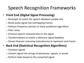
Speech Recognition Frameworks • Front End (Digital Signal Processing) • Resample to match the speech database sample rate • Break audio signal into overlapping frames • Perform frequency domain or linear prediction algorithms • Filter noise • Enhance speech characteristics in the signal • Transformations to match a reference signal database • Extract features removing redundancies to represent each frame • Back End (Statistical Recognition Algorithms) • Compare signals • Convert signal into strings of phonemes, signals, or words • Perform tasks based on the converted signal
Speech Frames Goal: Extract short-term signal features from speech signal frames • Breakup speech signal into overlapping frames • Why? • Speech is quasi-periodic, not periodic, because vocal musculature is always changing • Within a small window of time, we can assume constancy Frame Frame Frame Frame Frame shift Frame size Typical Characteristics 10-30 ms length 1/3 – 1/2 overlap
Speech Recognition Front End Assume resampling is already done Speech Frame Pre-emphasis windowing Temporal Features Spectral Analysis Frequency Features Enhance and Consolidate Features Feature Vector
Feature Extraction Goal: Remove redundancies by representing a frame by its feature “fingerprint” • Definitions • Feature: An attribute of a speech signal useful for decoding • Phoneme: The smallest phonetic unit that distinguishes words • Morpheme: The smallest phonetic unit that conveys meaning • Feature Extraction: Algorithm to convert a captured audio into a useable form for decoding • Feature Vector: List of values representing a given signal frame • Process • Signal Conditioning (digitizing a signal) • Signal Measurement (compute signal amplitudes) • Enhance (perform perceptual augmentations) • Conversion (Convert data into a feature vector) Challenge: Determine those features that are important?
Pre-emphasis • Human Audio • There is an attenuation of the audio signal loudness as it travels along the cochlea, which makes humans require less amplitudes in the higher frequencies • Speech high frequencies have initial less energy than low frequencies • De-emphasizing the lower frequencies compared to is closer to the way humans hear • Pre-emphasis Algorithm • Pre-emphasis recursive filter de-emphasizes lower frequencies • Formula: Y[i] = X[i] - (X[i-1] * δ) • 0.95 to 0.97 are common defaults for δ • 0.97 de-emphasizes lower frequencies more than 0.95
Pre-emphasis Filter Purpose: Reverse 6db/oct amplitudedecay in unvoiced soundsas frequencies increase y[i] = x[i] – x[i-1] * 0.95
Windowing • Problem: Framing a signal results in abrupt edges • Impact • There is significant spectral leakage in the frequency domain • Large side lobe amplitudes • Effect of Windowing • There are no abrupt edges • Minimizes side lobe amplitudes and spectral leakage • How?Apply a window formula in the time domain (which is a simple for loop) • Definitions • Frame: A small portion (sub-array) of an audio signal • Window: A frame to which a window function is applied
Window Types for Speech • Rectangular: wk = 1 where k = 0 … N • The Naïve approach • Advantage: Easy to calculate, array elements unchanged • Disadvantage: Messes up the frequency domain • Hamming: wk = 0.54 – 0.46 cos(2kπ/N-1)) • Advantage: Fast roll-off in frequency domain, popular for ASR • Disadvantage: worse attenuation in stop band • Blackman: wk = 0.42 – 0.5 cos(2kπ/(N-1)) + 0.08 cos(4kπ/(N-1)) • Advantage: better attenuation, popular for ASR • Disadvantage: wider main lobe • Hanning: wk = 0.5 – 0.5 cos(2kπ/N-1)) • Advantage: Useful for pitch transformation algorithms Multiply the window, point by point, to the audio frame
Create and Apply Hamming Window public double[] createHammingWindow(intfilterSize) { double[] window = new double[filterSize]; double c = 2*Math.PI / (filterSize - 1); for (int h=0; h<filterSize; h++) window[h] = 0.54 - 0.46*Math.cos(c*h); return window; } public double[] applyWindow(double[] window, double[] signal) { for(int i: window) signal[i] = signal[i]*window[i]; return samples; }
Rectangular Window Frequency Response Time Domain Filter
Temporal Features Advantages: less processing; usually easy to understand Examples • Energy • Zero-crossing rate • Auto correlation and auto differences • Pitch period • Fractal Dimension • Linear Prediction Coefficients Note: These features can directly be obtained from the raw signal
Signal Energy Useful to determine if a windowed frame contains a voiced speech • Calculate the short term frame energy Energy = ∑k=0,N (sk)2 where N is the size of the frame • Represent result in decibels relative to SPLdb = 10 log(energy) • Tradeoffs • If window is too small: too much variance • If window is too big: encompasses both voiced and unvoiced speech • Voiced speech has higher energy than unvoiced speech or silence • Changes in energy can indicate stressed syllables (loudness contour)
Zero Crossings • Eliminate a possible DC component, meaning every measurement is offset by some value • Average the absolute amplitudes ( 1/M ∑ 0,M-1sk ) • Subtract the average from each value • Count the number of times that the sign changes • ∑0,M-10.5|sign(sk)-sign(sk-1)|; where sign(x) = 1 if x≥0, -1 otherwise • Note: |sign(sk)-sign(sk-1)| equals 2 if it is a zero crossing Unvoiced speech tends to have higher zero crossing than background noise
Signal Correlation Determine self-similarity of a signal • Question: How well does a signal correlate with an offset version of itself? • Apply the auto-correlation formula R = ∑i=1,n-zxf[i]xf[i+offset]/∑i=1,Fxf[i]2 • Apply the auto-difference formula D = ∑i=1,n-zMath.abs(xf[i] - xf[i+offset]) • Either method is useful for determining the pitch of a signal. We would expect that R is maximum (and D minimum) when offset corresponds to that of the pitch period
Vocal Source • Speaker alters vocal tension of the vocal folds • If folds are opened, speech is unvoiced resembling background noise • If folds are stretched close, speech is voiced • Air pressure builds and vocal folds blow open releasing pressure and elasticity causes the vocal folds to fall back • Average fundamental frequency (F0): 60 Hz to 300 Hz • Speakers control vocal tension alters F0 and the perceived pitch Open Closed Pitch Period
Auto Correlation for pitch • Remove the DC offset and apply pre-emphasisxf[i] = (sf[i] – μf) – α(sf[i-1] – μf)where f=frame, μf = mean, α typically 0.96 • Apply the auto-correlation formula to estimate pitchRf[z] = ∑i=1,n-z xf[i]xf[i+z]/∑i=1,F xf[i]2M[k] = max(rf[z]) • Expectation: Voiced speech should produce a higher M[k] than unvoiced speech, silence, or noise frames • Notes: • We can do the same thing with Cepstrals • Auto-correlation complexity improved by limiting the Rf[z] values that we bother to compute
Fractal Dimension • Definition: The self-similarity of a signal • Comments • There are various methods to compute a signal’s self-similarity, which each lead to different results • Each method is empirical, not backed by mathematics • Some popular algorithms • Box Counting • Katz • Higuchi • Importance: We would expect that the self-similarity of speech, because it is constrained by the larynx and vocal tract, to be different than that of background noise
Box Counting Algorithm Assume signal[i] is an array of audio amplitudes, where each sample represents t milliseconds delta = 1 FOR i = 0 to S delta = 2^i Cover the curve with rectangles: h = signal[i+delta] – signal[i], w = delta * t Fractal[i] = count of rectangles needed to cover the curve Perform a linear regression on the Fractal array The slope of the best fit line is the fractal dimension
Linear Regression • Set of points: (x1,y1), (x2,y2), … (xN,yN) • Equations: Find b0 + b1x1 that minimizes errors where Yi = b0+b1xi+ei • Goal:Find slope b1 of the best fit line • Assumption: the expected value (mean) of the errors is zero • Note: X’ is transpose of X, -1 is inverse
Best Fit Slope of x amplitudes Assuming that the x points are 1, 2, 3, … Method returns b1of y = b0 + b1x bestFit(double[] y) { int MAX = y.length; // Compute the X’X matrix (aij) double a11 = MAX*(MAX+1)*(2*MAX+1)/6; // ∑ xi2 = d (a11 of inverse matrix) double a12 = MAX * (MAX + 1) / 2; // ∑ xi = b = c double a21 = a12, a22 = MAX; // a (a22 of the inverse matrix) // Compute ∑yi and sum ∑ xi * yi bi = X’y double sumXY=0, sumY=0; for (int i=0; i<MAX; i++) { sumXY += (i+1) * y[i]; sumY += y[i]; } // Return (X’X)-1 * X’y, where (X’X)-1 is the inverse of X’X double numerator = -a12*sumY + a22*sumXY ;// -c*sumXY+a*sumY double denominator = a11 * a22 – a12 * a12; // ad - bc return (denominator == 0) ? 0 : numerator / denominator; } Note:
Katz Fractal Dimension Dimension = log(sum of lengths)/log(largest distance from the first point) double katz(double[] x) { int N = x.length; if (N<=1) return 0; double L=0, diff=0, D=0; for (int i=1; i<x.length; i++) { L += Math.abs(x[i] - x[i-1]); diff = Math.abs(x[0] – x[i]); if (diff > D) D = diff; } double log = Math.log10(N-1); return (d==0)?0:log/(Math.log10(d/L)+log); } • L = ∑ xi – xi-1 (sums adjacent lengths) • max, min = from first point • Katz normalizes log(L)/log(D)) to use log(L/d)/log(D/d) • Final formulalog(L/d)/log(D/d) = log(N - 1) / log(D/(L/(N-1))) = log(N-1) / (log(D/m) + log(N-1)) • Notes • N-1 because there are N-1 intervals with a signal of N points • L / d = L / (L/(N-1)) = N-1
Higuchi Fractal Dimension (cont) public double higuchi (double[] x) { int MAX = x.length/4; double[] L = new double[MAX]; for (int k=1; k<=MAX; k++) { L[k-1] = Lk(x, k)/k; } // Find least squares linear best fit of L double slope = bestFit(L, MAX) + 1e-6; return Math.log10(Math.abs(slope)); } double Lk(double[] x, int k) { double sum = 0; for (int m=1; m<=k; m++) { sum += LmK(x, m, k); } return sum / k; } double LmK(double[] x, int m, int k) { int N = x.length; double sum = 0; for (int i=1; i<=(N-m)/k; i++) { sum += Math.abs(x[m-1+i*k]-x[m-1+(i-1)*k]); } return sum * (N - 1) / ((N - m)/k * k); }
Linear Prediction Coding (LPC) • Originally developed to compress (code) speech • Although coding pertains to compression, LPC has much broader implications • LPC is equivalent to the tubal model of the vocal tract model • LPC can be used as a filter to reduce noise (Wiener filter) from a signal • A speech frame can be approximated with a set of LPC coefficients • one coefficient per 1k of sample rate + 2 • Example: For a 10k sample, 12 LPC coefficients are sufficient • LPC speech recognition is somewhat noise resilient
Illustration: Linear Prediction {1, 2, 3, 4, 5, 6, 7, 8, 9, 10, 11, 12, 13, 14, 15, 16} Goal: Estimate yn using the three previous values yn ≈ a1 yn-1 + a2 yn-2 + a3 yn-3 Three ak coefficients, Frame size of 16, 3 coefficients Thirteen equations and three unknowns Note: No solutions, but LPC finds coeffients with the smallest error
Solving n equations and n unknowns • Gaussian Elimination • Complexity: O(n3) • Successive Iteration • Complexity varies • Cholesky Decomposition • More efficient, still O(n3) • Levenson-Durbin • Complexity: O(n2) • Works for symmetric Toplitz matrices Definitions for any matrix, A Transpose (AT): Replace aij by aji for all i and j Symmetric: AT = A Toplitz: Diagonals to the right all have equal values
Covariance Example Note: φ(j,k) = ∑n=start,start+N-1 yn-kyn-j • Signal: {…, 3, 2, -1, -3, -5, -2, 0, 1, 2, 4, 3, 1, 0, -1, -2, -4, -1, 0, 3, 1, 0, …} • Frame: {-5, -2, 0, 1, 2, 4, 3, 1}, Number of coefficients: 3 • φ(1,1) = -3*-3 +-5*-5 + -2*-2 + 0*0 + 1*1 + 2*2 + 4*4 + 3*3 = 68 • φ(2,1) = -1*-3 +-3*-5 + -5*-2 + -2*0 + 0*1 + 1*2 + 2*4 + 4*3 = 50 • φ(3,1) = 2*-3 +-1*-5 + -3*-2 + -5*0 + -2*1 + 0*2 + 1*4 + 2*3 = 13 • φ(1,2) = -3*-1 +-5*-3 + -2*-5 + 0*-2 + 1*0 + 2*1 + 4*2 + 3*4 = 50 • φ(2,2) = -1*-1 +-3*-3 + -5*-5 + -2*-2 + 0*0 + 1*1 + 2*2 + 4*4 = 60 • φ(3,2) = 2*-1 +-1*-3 + -3*-5 + -5*-2 + -2*0 + 0*1 + 1*2 + 2*4 = 36 • φ(1,3) = -3*2 +-5*-1 + -2*-3 + 0*-5 + 1*-2 + 2*0 + 4*1 + 3*2 = 13 • φ(2,3) = -1*2 +-3*-1 + -5*-3 + -2*-5 + 0*-2 + 1*0 + 2*1 + 4*2 = 36 • φ(3,3) = 2*2 +-1*-1 + -3*-3 + -5*-5 + -2*-2 + 0*0 + 1*1 + 2*2 = 48 • φ(1,0) = -3*-5 +-5*-2 + -2*0 + 0*1 + 1*2 + 2*4 + 4*3 + 3*1 = 50 • φ(2,0) = -1*-5 +-3*-2 + -5*0 + -2*1 + 0*2 + 1*4 + 2*3 + 4*1 = 23 • φ(3,0) = 2*-5 +-1*-2 + -3*0 + -5*1 + -2*2 + 0*4 + 1*3 + 2*1 = -12
Auto Correlation Example Note: φ(j,k)=∑n=0,N-1-(j-k) ynyn+(j-k)=R(j-k) • Signal: {…, 3, 2, -1, -3, -5, -2, 0, 1, 2, 4, 3, 1, 0, -1, -2, -4, -1, 0, 3, 1, 0, …} • Frame: {-5, -2, 0, 1, 2, 4, 3, 1}, Number of coefficients: 3 • R(0) = -5*-5 + -2*-2 + 0*0 + 1*1 + 2*2 + 4*4 + 3*3 + 1*1 = 60 • R(1) = -5*-2 + -2*0 + 0*1 + 1*2 + 2*4 + 4*3 + 3*1 = 35 • R(2) = -5*0 + -2*1 + 0*2 + 1*4 + 2*3 + 4*1 = 12 • R(3) = -5*1 + -2*2 + 0*4 + 1*3 + 2*1 = -4 Assumption: all entries before and after the frame treated as zero
Voice Activity Detection (VAD) • Problem: Determine if voice is present in an audio signal • Issues: • Without VAD, ASR accuracy degrades by 70% in noisy environments. VAD has more impact on robust ASR than any other single component • Using only energy as a feature, loud noise looks like speech and unvoiced speech as noise • Applications: Speech Recognition, transmission, and enhancement • Goal: extract features from a signal that emphasize differences between speech and background noise • Evaluation Standard:Without an objective standard, researchers cannot scientifically evaluate various algorithms H.G. Hirsch, D. Pearce, “The Aurora experimental framework for the performance evaluation of speech recognition systems under noisy conditions,” Proc. ISCAITRW ASR2000, vol. ASSP-32, pp. 181-188, Sep. 2000
Samples of VAD approaches • Noise • Level estimated during periods of low energy • Adaptive estimate: The noise floor estimate lowers quickly and raises slowly when encountering non-speech frames • Energy: Speech energy significantly exceeds the noise level • Cepstrum Analysis(Covered later in the term) • Voiced speech contains F0 plus frequency harmonics that show as peaks in the Cepstrum • Flat Cepstrums, without peaks, can imply door slams or claps • Kurtosis:Linear predictive coding voiced speech residuals have a large kurtosis
Statistics: Moments • First moment - Mean or average value: μ = ∑i=1,N si • Second moment - Variance or spread: σ2 = 1/N∑i=1,N(si - μ)2 • Standard deviation – square root of variance: σ • 3rd standardized moment- Skewness: γ1 = 1/N∑i=1,N(si-μ)3/σ3 • Negative tail: skew to the left • Positive tail: skew to the right • 4th standardized moment – Kurtosis: γ2 = 1/N∑i=1,N(si-μ)4/σ4 • Positive: relatively peaked • Negative: relatively flat
Statistical Calculations (Excel Formulas) for (int frame=0; frame< N; frame++) // Total a given feature over all frames { totals[MEAN][feature] += features[frame][offsets[feature]]; } totals[MEAN][feature]/= N; } // Compute mean double delta, factor, stdev; for (int frame=0; frame < N; frame++) {delta = (features[frame][offsets[feature]] - totals[MEAN][feature]); totals[VARIANCE][feature] += delta * delta; totals[SKEW][feature] += Math.pow(delta, 3); totals[KIRTOSIS][feature] += Math.pow(delta, 4); } totals[VARIANCE][feature] = totals[VARIANCE][feature] /= N - 1; totals[STD][feature] = stdev = Math.sqrt(totals[VARIANCE][feature]); factor = 1.0 * N / ((N-1)*(N-2)); totals[SKEW][feature] = factor * totals[SKEW][feature] / Math.pow(stdev, 3); factor = 1.0 * N * (N+1) / ((N-1)*(N-2)*(N-3)); totals[KIRTOSIS][feature] = factor*totals[KIRTOSIS][feature] / Math.pow(stdev,4); factor = 3.0 * (N-1)*(N-1) / ((N-2)*(N-3)); totals[KIRTOSIS][feature] -= factor;
Rabiner’s Algorithm • Uses energy and zero crossings • Reasonably efficient • Calculated in the time domain • Calculates energy/zero crossing thresholds on the first quarter second of the audio signal (assumed to be noise frames without speech) • Is reasonable accurate when the signal to noise ratio is 30 db or higher • Assumes high energy frames contain speech, and a significant number of surrounding frames with high zero crossing counts represent unvoiced consonants
Entropy is a possible VAD feature • Entropy: Bits needed to store information • Formula: Computing the entropy for possible values: Entropy(p1, p2, …, pn) = - p1lg p1 – p2lg p2 … - pn lg pn • Where pi is the probability of the ith value log2x is logarithm base 2 of x • Examples: • A coin toss requires one bit (head=1, tail=0) • A question with 30 equally likely answers requires∑i=1,30-(1/30)lg(1/30) = - lg(1/30) = 4.907
Use of Entropy as VAD Metric FOR each frame Apply an array of band pass frequency filters to the signal FOR each band pass frequency filter output energy[filterNo] = ∑i=bstart,bendx[i]2 IF this is an initial frame, noise[filterNo] = energy[filterNo] ELSEspeech[filterNo]= energy[filterNo] – noise[filterNo] Sort speech arrayand use subset of MAX filters with max speech[filterNo] values FORi = 0 to MAX DOtotal += speech[i] FORi = 0 to MAX DO entropy += speech[i]/total * log(speech[i]/total) IF entropy > threshold THEN return SPEECH ELSE return NOISE Notes: • We expect higher entropy in noise; speech frames should be structured • Adaptive enhancement: adjust noise estimates whenever encountering a frame deemed to be noise. noise[filterNo] = noise[filterNo] * α + energy[filterNo] * (1 -α) where 0<=α<=1
Unvoiced Speech DetectorFilter Bank Decomposition • EL,0 = sum of all level five energy bands • EL,1 = sum of first four level 4 energy bands • EL,2 = sum of last five level 4 energy bands + first level 3 energy band • IF EL,2 > EL,1 > EL,0 and EL,0/EL,2 < 0.99, THEN frame is unvoiced speech
G 729 VAD Algorithm • Importance: An industry standard and a reference to compare new proposed algorithms • Overview • A VAD decision is made every 10 ms • Features: full band energy, the low band energy, the zero-crossing rate, and a spectral frequency measure. • A long term average of frames judged to not contain voice • VAD decision: • compute differences between a frame and noise estimate. • Adjust difference using average values from predecessor frames to prevent eliminating non-voiced speech • IF differences > threshold, return true; ELSE return false
Non-Stationary Click Detection Stationary noise has a relatively constant noise spectrum, like a background fan • Compute the standard deviation (σ) of a frame’s LPC residue • Algorithm FOR each frame (f) Perform the Linear prediction with C coefficents (c[i]) lpc= Convolution of the frame using the c[i] as a filter residue energy residue[i] = |lpc[i] – f[i]2 Compute the standard deviation of the residue (σ) IF K σ > threshold, where K is an empirically set gain factor • Approach 1: Throw away frames determined to contain clicks • Approach 2: Use interpolation to smooth the residue signal of clicks Definition: Residue – difference between the signal and the LPC generated signal
Experiment • Approach 1: Throw away click frames • Approach 2: Interpolate click frames Music without clicks Music clicks
LPC Features as a front end • Assumptions • LPC models the vocal tract as a P order all-pole IIR filter • Future discrete signal samples are functions of the previous ones • The speech signal is purely linear • Coefficients: Generally eight to fourteen LPC coefficients are sufficient to represent a particular block of sound samples • Disadvantage: Linear prediction coefficients tend to be less stable other methods (ex: Cepstral analysis) • Enhancement: Perceptual Linear Prediction uses bot frequency and time domain data. The result is comparable to Cepstral analys.
The LPC Spectrum Perform a LPC analysis Find the poles Plot the spectrum aroundthe z-Plane unit circle What do we find concerning the LPC spectrum? Adding poles better matches speech up to about 18 for a 16k sampling rate The peaks tend to be overly sharp (“spiky”) because small radius changesgreatly alters pole skirt widths in the z-plane
Filter Bank Front End • The bank consists of twenty to thirty overlapping band pass filters spread along the warped frequency axis • Represent spectrum with log-energy output from filter bank • Each frequency bank F handles frequencies from f-i to f+i or individual ranges of frequencies that models the rows of hair bands in the cochlea • The feature data is an array of energy values obtained from each filter • Result: Good idea, but it has not proven to be as effective as other methods
Warped band pass filter set Mel frequency warping
Time Domain Filtering • Band Pass • Filter frequencies below the minimum fundamental frequency (F0) • Filter frequencies above the speech range (≈4kHz) • Linear smoother and median of five filters • Used in combination to smooth the pitch contour • Derivative (slope) filter • Measure changes in a given feature from one frame to another • Tends to reduce the effects of noise in ASR • Noise Removal: Separate set of slides
Band Pass Filters ACORNS uses Butterworth and Window Sync filters • Butterworth • Advantages: • IIR filter, which is fast • minimal ripple • Disadvantage: slow transition • Window Sync • Advantage: quick transition • Disadvantages • FIR filter, which is slow • Ripples in the pass band • Many other filters with various advantages and disadvantages. Open source code for these exist.
Median of Five private void medianOfFive(int feature) { double median, save, middle, out[] = new double[features.length]; for (int frame=2; frame<features.length - 2; frame++) { median = features[frame+2][feature]; save = features[frame+1][feature]; if (median > save) { median = features[frame+1][feature]; save = features[frame+2][feature]; } if (features[frame-2][feature]<features[frame-1][feature]) { if (features[frame-2][feature]>median) median= features[frame-2][feature]; if (features[frame-1][feature]<save) save = features[frame-1][feature]; } else { if (features[frame-1][feature]>median) median= features[frame-1][feature]; If (features[frame-2][feature]<save) save = features[frame-2][feature]; } middle = features[frame][feature]; if ((save - middle) * (save-median) <= 0) median = save; if ((middle - save) * (middle - median) <= 0) median = middle; out[frame] = median; }
Linear Smoother private void linearSmoother(int feature) { if (features==null) return; double[] out = new double[features.length]; for (int frame = 2; frame<features.length; frame++) { out[frame] = features[frame][feature]/4 + features[frame-1][feature]/2 + features[frame-2][feature]/4; } }