Mastering Present Value Computation in Finance
Learn to compute present values for investments and annuities. Understand compounding, discounting, and geometric series in financial valuation.

Mastering Present Value Computation in Finance
E N D
Presentation Transcript
Present Value Professor Thomas Chemmanur
Review of Present Value Computation All of you must be somewhat familiar with computing present values from previous classes. Computing present value is at the core of all valuation problems in finance. To ensure you are comfortable with present value computation, I will therefore briefly review this material. i. Future value of a single amount where F is the future value of an investment P after n periods, at a rate of return r per period. The term (1 + r)n is tabulated, and is often denoted by FVIFn,r. 2
Review of Present Value Computation ii. Present value of a single amount. where P is the present value of a single amount F to be received n periods from now, if the opportunity cost of capital is r per period. The term [1/(1 + r)n] is tabulated, and is often denoted by PVIFn,r. iii. Future Value of an annuity. An annuity is a stream of cash flows where the cash flow in each period is the same. Consider the following three period annuity; t = 0 t = 1 t =2 t = 3 Date: Cash Flow: A A A 3
Review of Present Value Computation Note: Throughout this course, we will use this distinction between dates and periods. Let us first compute the future value (i.e., the value at the end of the last period: i.e., at t=3) of this three period annuity. Using the formula (1) on each individual cash flow, and adding value at t = 3 (remember, we can add values at the same date): F = A + A(1 + r) + A(1 + r)2 Notice that the index on the last term is 3 - 1 = 2. Generalizing to the n period case, the future value of an n period annuity is, F = A + A(1 + r) + A(1 + r)2 + A(1 + r)3 +.....+ A(1 + r)n-1. = A [ 1 + (1 + r) + (1 +r)2 + (1 + r)3 +....+ (1 + r)n-1 ] 4
Review of Present Value Computation The series inside the square brackets is a geometric series, with common ratio (1 + r). Making use of the formula for the sum of a geometric series, the term in the square brackets can be shown to be equal to Thus, The term in square brackets is tabulated, and is often denoted by FVIFAn,r. iv. Present value of an annuity. Using the same three period cash flow stream above as an example, the present value of the three period annuity (i.e., value at t=0) is, 5
Review of Present Value Computation Generalizing to the n period case as before, The series in the square brackets is a geometric series with common ratio 1/(1 + r). Using the formula for the sum of a geometric series, this series sums to 6
Review of Present Value Computation This gives, The term in square brackets is tabulated, and is denoted by PVIFAn,r. If the number of periods, n, goes to infinity, (7) can be shown to reduce to which is the present value of a perpetual annuity or perpetuity. 7
Review of Present Value Computation v. Compounding and discounting more than once in a given period. Sometimes the period over which the data is given may not be the period over which compounding is done. Eg. Let R be the interest rate per year, T be the number of years. a) Future value of an amount P compounded half-yearly after T years at R is given by converting this data to correspond with the compounding period: n = number of effective periods = 2T in this example. r = interest rate per effective period = R/2. Then the future value is given by plugging in these values into (1). Generalizing to the case where compounding is done m times a year, r = R/m, and n = mT. Using these in (1), 8
Review of Present Value Computation b) Similarly, the present value of an amount F, T years in the future, if discounting is done m times a year at a rate of return of R per year is, vi. Continuous compounding and discounting. Consider the case when m goes to infinity, i.e., compounding is done continuously. Taking the limit of (9) as , 9
Review of Present Value Computation The present value of an amount F to be received T years from now, where discounting is done continuously at the rate of return R per year is easily obtained from (11) as, 10
Appendix: Sum of a geometric series. Consider a series of terms of the form 1, k, k2, k3,....kn-1. Each successive term is k times the previous one; k is therefore called the common ratio. The sum of all the above terms can be shown to be equal to, S = 1 + k + k2 + k3 +...+ kn-1 = [(kn - 1)/(k-1)]. Whenever we see a series of the above form, we can sum it using the above formula, by setting k equal to the common ratio of that particular series. Consider now the case where the number of terms in the series,. If k > 1, each successive term is larger than the previous one, and . However, in the special case where k < 1, we can show that the sum is given by, S = 1/(1 - k). 11