Routing in Wireless and Adversarial Networks
410 likes | 569 Vues
Routing in Wireless and Adversarial Networks. Christian Scheideler Institut für Informatik Technische Universität München. Routing. Path selection Scheduling Admission control. B. A. Classical Routing Theory. Given a path collection with

Routing in Wireless and Adversarial Networks
E N D
Presentation Transcript
Routing in Wireless and Adversarial Networks Christian Scheideler Institut für Informatik Technische Universität München
Routing • Path selection • Scheduling • Admission control B A
Classical Routing Theory Given a path collection with • congestionC (max. number of paths over edge) and • dilationD (max. length of a path) find (near-)optimal schedule for packets.
Classical Routing Theory Leighton, Maggs, Rao 88: There is a schedule with O(C+D) runtime. Also for non-uniform edges [Feige & S 98] Since then many randomized online protocols with runtime ~O(C+D) w.h.p. Basic techniques: random delays or ranks
Classical Routing Theory Extensions faulty and wireless networks. Adler & S 98: • G=(V,E) with probabilities p:E ! [0,1] • H=(V,E) with latencies l(e)=1/p(e) • Valid routing schedule of length T for H can be simulated in G in time O(T log L + L log n), w.h.p.; L: max. latency
Scheduling Classical model: batch-like scheduling More relevant models: • Stochastic injection models(packets are continuously injected using Poisson distribution or Markov chains) • Adversarial queueing theory(introduced by Borodin et al. 96)
Adversarial Queueing Theory Basic model: • Static network G=(V,E) • (w,)-bounded adversary continuously injects packets subject to the condition that for all edges e and all time intervals of length w, it injects at most w packets with paths containing e • All packets have to be delivered (<=1)
Adversarial Queueing Theory Basic results: • Universal stabilityand instability of various queueing disciplines (FIFO, SIS, LIS, NTO,…) • Universal stability of networks
Adversarial Queueing Theory Networks with time-varying channels: • Packet injections and edges under adversarial control • Andrews and Zhang 04: Variant of NTO is universally stable in this model
Adversarial Routing Theory Paths are not given to system: • Aiello, Kushilevitz, Ostrovsky, Rosen ’98:local load balancing techniques can be used to keep queues bounded
Adversarial Routing Theory Paths are not given to system: • Awerbuch, Brinkmann & S ’03:local load balancing technique with bounded queues also handles admission,works even for adversarial networks
Adversarial Routing Theory Paths are not given to system: • Awerbuch, Brinkmann & S ’03:load balancing technique with O(L/) times buffer space of OPT is (1+)-competitive w.r.t. throughput; L: max path length
Path Selection Problems: - packet-based paths: slow delivery - destination-based paths: congestion Better:source-based path selection (MPLS: Multiprotocol Label Switching)
Path Selection Classical work: path selection strategies for specific networks (n£n-mesh) B x-y routing A
Path Selection x-y routing: ~worst-case optimal congestion and dilation for permutation routing B x-y routing A
Path Selection x-y routing: far from optimal in general t3 t2 t1 x-y routing s3 s2 s1
Path Selection Trick: use hierarchical randomized routing. (log n)-competitive for any problem t3 t2 t1 s3 s2 s1
Oblivious Path Selection Räcke 02: For any network with edge capacities, path collections for random path selection can be set up for every source-destination pair s.t. the expected congestion of routing any routing problem is O(log3 n)-competitive. Best bound [HHR03]:~O(log2 n) 1/2 1/4 1/4
Oblivious Path Selection Also works well for certain dynamic net-works for peer-to-peer systems. Trick:continuous-discrete approach • route in virtual space • nodes partition virtual space among them
Oblivious Path Selection Does not work well for wireless, unknown or adversarial networks (e.g., unstructured P2P systems with adversarial presence)
Adaptive Path Selection Basic Idea: Garg & Könemann 98 Multicommodity flow problem: collection of commodities (source, dest., demand) • Solution 1: use LP • Solution 2:combinatorial approach (path packing using primal-dual approach)
Garg-Könemann Framework Problem:MCF (maximum concurrent flow problem), i.e., given commodities with demands di, find flows of value di for commodities s.t. maxe fe/ce minimized Goal: find (1+)-approximate solution via path packing
Garg-Könemann Framework Initially, fei=0 for all commodities i and edges e Algorithm runs in T=ln m/2phases, routes a flow of di/T for each commodity i in each phase A phase consists of several steps In each step, flows augmented simultaneously subject to two constraints: • (1+)-shortest paths constraint, using edge lengths le = mconge//ce with conge = fe/ce • step-size constraint: le <= le(which implies fe <= 2 ce/ln m)
Garg-Könemann Framework Original Garg-Könemann approach: • Route commodities in round-robin fashion, one commodity per step) #steps depends linearly on #commidities Awerbuch, Khandekar and Rao 07: • Route commodities simultaneously in each step using capacities cei = 2 fei/log m for comm i)multiplicative-increase strategy, faster conv
Garg-Könemann Framework Awerbuch, Khandekar and Rao 07:runtime O(L log3 m log k)L: max flow length, k: #commodities • L small (hypercube): fast convergence • Lalways boundable by expansion of net(flow shortening lemma [Kolman & S 02])
Oblivious vs. Adaptive Congestion for arbitrary routing problems in hypercubic networks: • Oblivious path selection:(log n)-competitive, paths instantly, update of path system complicated • Adaptive path selection:(1+)-competitive, paths in polylog comm rounds, continuous updates easy
Adaptive Path Selection Problem: previous approaches not stateless resp. self-stabilizing Awerbuch and Khandekar 07: • Adaptive path selection strategy that only needs to know current state • Fast convergence through greedy strategy based on multiplicative increase, additive decrease
Adversarial Path Selection Scenario I: Adversaries part of network, but path along honest nodes available A B
Adversarial Path Selection Basic approach:A fixes a path from A to B. Path does not work: A identifies bad edge. A B
Adversarial Path Selection Identification of bad edge: Acknowledgements via binary search A B
Adversarial Path Selection Maximum number of attempts: m (# edges) Either successful or edge killed. A B
Adversarial Path Selection Improvement: use recommendations If neighbor knows better, suggests a diff path !collaborative learning A B
Adversarial Path Selection Scenario II: All nodes adversarial. Awerbuch and Kleinberg 04: Learns best static path in hindsight 1 10 2 2 A 7 1 3 2 5 3 B 4
Adversarial path selection Model: • There is a set S of static strategies (paths) • Algorithm A interacts with adversary for T steps • In each step j, the adversary picks a cost function cj:S ! IR and A picks a random strategy xj2 S • Only cost of chosen strategy revealed to A • The regret of the algorithm A is defined asR(A) = E[j cj(xj) – minx 2 Sj cj(x)]
Adversarial Path Selection Awerbuch and Kleinberg: • Regret of O(T2/3 C m5/3) against oblivious adversaryC: maximum cost difference, m: #edges • Regret of O(T2/3 C7/3 m1/3) against adaptive adversary Regret does not depend on |S| !
Adversarial Path Selection Otto von Bismarck:Fools learn from experience; wise men learn from the experience of others. Only collaborative learning result due to Awerbuch and Hayes 07, who study the dynamic regret for |S|=2:R(A) = avga E[j cj(xj) – jminx 2 S cj(x)]
Adversarial Path Selection Awerbuch and Hayes 07: • N agents, n of which are honest • In each round, agents make decisions in a fixed order, report the costs incurred • Costs are either 0 or 1 • Dynamic regret:O(log N2 + T/n)log2 N: rounds to figure out whom to trustT/n: just one mistake per round
Adversarial Path Selection Scenario III: Network topology unknownbut position of destination known • Geometric spanners (wireless networks) • Navigable graphs (small world)pioneered by Kleinberg 96 How to design self-stabilizing processes?
Adversarial Path Selection Scenario IV: Network topology unknown and position of destination unknown! discovery via flooding A B
Open Problems • Scheduling: non-uniform problems • Path selection: many open problems left • Collaborative learning approaches particularly interesting