Wavelet Transform for Image Data Compression
Wavelet Transform for Image Data Compression . 王 隆 仁. Contents. Introduction Transforms Wavelet Analysis Harr Wavelets Subband filtering scheme Further Research. I. Introduction.

Wavelet Transform for Image Data Compression
E N D
Presentation Transcript
Contents • Introduction • Transforms • Wavelet Analysis • Harr Wavelets • Subband filtering scheme • Further Research
I. Introduction • Image data compression can be used to reduce the storage requirement of a fixed memory and decrease the time needed to transfer image data between networks. • Compression can be achieved by transforming the data, projecting it on a basis of functions, and then encoding this transform.
Because of the nature of the image signal and the mechanisms of human vision, the transform used must accept nonstationarity and be well localized in both the space and frequency domain. • To avoid redundancy, the transform must be at least biorthogonal and lastly, in order to save CPU time, the corresponding algorithm must be fast. The wavelet transform satisfies each of these conditions.
The two-dimensional wavelet transform defined by Meyer and Lemarie, together with its implementation as described by Mallat, satisfies each of these conditions. • The wavelet transform cuts up the image into a set of subimages with different resolutions corresponding to different frequency bands. • One compression approach is based on a wavelet transform and a vector quantization coding scheme.
II. Transforms • The transform of a signal (a vector) is a new repre-sentation of that signal. • The transform can be divided into three groups : 1. Lossless (orthogonal) transforms (orthogonal and unitary matrices) 2. Invertible (biorthogonal) transforms (invertible matrices) 3. Lossy transforms (not invertible)
A lossless unitary transform is like rotation. The transformed signal has the same length as the original. The same signal is measured along new perpendicular axes. ( Example : FFT, DCT, … ) • For biorthogonal transforms, lengths and angles may change. The new axes are not necessarily per-pendicular, but no information is lost. Perfect reconstruction is still available. It just inverts. • Orthogonal wavelets give orthogonal matrices and unitary transforms, biorthogonal wavelets give invertible matrices and perfect reconstruction.
These transforms don’t remove any information or any noise, they just move it around --- aiming to separate out the noise and decorrelate the signal. • The irreversible step is to destroy small components, as we do below in “compression”. The invertible is lost. • The transform from x to y is executed by a matrix :
The matrix that recovers x from y is changed only by the factor 1/2 : • For example, if x(0)=1.2, x(1)=1.0, x(2)=-1.0 and x(3)=-1.2 then y(0)=2.2, y(1)=0.2, y(2)=-2.2 and y(3)=0.2. (compute sums and differences) • y(1) and y(3) are much smaller than y(0) and y(2). If we cancel the small numbers y(1) and y(3) --- the compressed signal yc is
yc(0)=2.2, yc(1)=0, yc(2)=-2.2 and yc(3)=0. • Those numbers 0.2 were below our threshold. In the compressed yc they are gone. • Finally, the signal xc reconstructed from yc, xc(0)=1.1, xc(1)=1.1, xc(2)=-1.1 and xc(3)=-1.1 --- the small difference between x(0) and x(1) is lost. • A key idea for wavelets is concept of “scale”. Sums and differences of neighbors are at the finest scale. This is recursion --- the same transform at a new scale. It leads to a multiresolution of the original signal. Averages and details will appear at different scales.
The wavelet formulation keeps the differences y(1) and y(3) at the finest level, and iterates only on y(0) and y(2). • Iteration means sum and difference of the transform: z(0)=y(0)+y(2)=0 and z(2)=y(0)-y(2)=4.4. • At this level there is extra compression. One component z(2) now does most of the work of the original four. • The wavelet transform is z(0)=0, y(1)=0.2, z(2)=4.4 and y(3)=0.2. The compressed signal is zc(0)=0, yc(1)=0, zc(2)=4.4 and yc(3)=0.
sums z(0) sums y(0), y(2) differences z(2) x differences y(1), y(3) • The multilevel transforms by recursion is clear in a flow-graph : • This is two-step wavelet transform. It is invertible. • To draw the flow-graph of the inverse, just reverse the arrows.
III. Wavelet Analysis • Wavelets are functions generated from one single function by dilations and translations where is a one-dimension variable, are called wavelets, is called mother wavelet, is a scale or frequency, and is corresponding time-domain function.
The definition of wavelets as dilates of one function means that high frequency wavelets correspond to or narrow width, while low frequency wavelets have or wider width. • A typical wavelet is compressed times and shifted times. Its formula is • At a given resolution of a signal or an image, the scaling functions are a basis for the set of signals.
signal at level j (local average) signal at level j+1 + details at level j (local differences) • The level is set by , and the time steps at that level are . The new details at level are represented by the wavelets . Then the smooth signal plus the details, the plus the , combine into a multiresolution of the signal at the finer level . • Averages come from the scaling functions, details come from the wavelets:
Vj = scaling space at level j Vj+1 = scaling space at level j+1 Wj = wavelet space at level j • That is multiresolution for one signal. When we apply it to all signals, we have multiresolution for spaces of functions: • This idea of multiresolution is absolutely basic to wavelet analysis.
The wavelet decomposition is • The constitute an orthonormal basis, so that • The are orthonormal, one denotes by the space spanned by the ; these spaces are successive approximation spaces,
For each , the span a space which is exactly the orthogonal complement in of ; the coefficients , therefore, describe the information lost when going from an approximation of with resolution to the coarser approximation with resolution • This is translated into the following algorithms :
where and • In fact the are coefficients characterizing the projection of onto . • If the function is given in sampled form, then one can take these samples for the highest order resolution approximation coefficients , and (1) describes a subband coding algorithm on these sampled values, with low-pass filter and high-pass filter .
Because of their association with orthonormal wavelet bases, these filters give the exact reconstruction, i.e. :
IV. Haar Wavelets • Scaling functions 1. Haar scaling function is defined by and is shown in Fig. 1. Some examples of its translated and scaled versions are shown in Fig. 2-4. 2. The two-scale relation for Haar scaling function is
Fig.1: Haar scaling function (x). Fig.2: Haar scaling function (x-1). Fig.3: Haar scaling function (2x). Fig.4: Haar scaling function (2x-1).
Wavelets 1. The Haar wavelet (x) is given by and is shown in Fig. 5. 2. The two-scale relation for Haar wavelet is
Decomposition relation 1. Both of the two-scale relation together are called the reconstruction relation. 2. The decomposition relation can be derived as follows.
COLUMNS ROWS Image corresponding to the low resolution level m h 2 h 2 Initial image corresponding to the resolution level m-1 g 2 Detail images corresponding to the resolution level m h 2 g 2 g 2 h Convolve with low-pass filter 2 Downsampling or decimation g Convolve with high-pass filter V. Subband filtering scheme Fig. 6: One stage in a multiscale image decomposition.
COLUMNS ROWS Image corresponding to the low resolution level m 2 2 Reconstructed image resolution level m-1 2 Detail images resolution level m 2 2 2 X Convolve with filter X 2 Upsampling Fig. 7: One stage in a multiscale image reconstruction.