Multiplicative Bounds for Metric Labeling

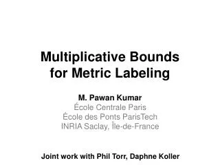
1. Multiplicative Boundsfor Metric Labeling M. Pawan Kumar ÉcoleCentrale Paris Écoledes PontsParisTech INRIA Saclay, Île-de-France Joint work with Phil Torr, Daphne Koller

2. Energy Minimization Variables V= { V1, V2, …, Vn}

3. Energy Minimization Variables V= { V1, V2, …, Vn}

4. Energy Minimization θab(f(a),f(b)) θb(f(b)) θa(f(a)) Va Vb minf E(f) + Σ(a,b)θab(f(a),f(b)) = Σaθa(f(a)) Labels L= { l1, l2, …, lh} Variables V= { V1, V2, …, Vn} Labeling f: { 1, 2, …, n}  {1, 2, …, h}

5. Energy Minimization Va Vb minf E(f) + Σ(a,b)θab(f(a),f(b)) = Σaθa(f(a)) NP hard

6. Metric Labeling Va Vb minf E(f) + Σ(a,b)θab(f(a),f(b)) = Σaθa(f(a))

7. Metric Labeling Va Vb minf E(f) + Σ(a,b)sabd(f(a),f(b)) = Σaθa(f(a)) d(.) is a metric distance function sabis non-negative NP hard Low-level vision applications

8. Approximate Algorithms • Minka. Expectation Propagation for Approximate Bayesian Inference, UAI, 2001 • Murphy et al. Loopy Belief Propagation: An Empirical Study, UAI, 1999 • Winn et al. Variational Message Passing, JMLR, 2005 • Yedidiaet al. Generalized Belief Propagation, NIPS, 2001 • Besag. On the Statistical Analysis of Dirty Pictures, JRSS, 1986 • Boykov et al. Fast Approximate Energy Minimization via Graph Cuts, PAMI, 2001 • Komodakis et al. Fast, Approximately Optimal Solutions for Single and Dynamic • MRFs, CVPR, 2007 • Lempitsky et al. Fusion Moves for Markov Random Field Optimization, PAMI, 2010 • Chekuri et al. Approximation Algorithms for Metric Labeling, SODA, 2001 • Goemanset al. Improved Approximate Algorithms for Maximum-Cut, JACM, 1995 • Muramatsuet al. A New SOCP Relaxation for Max-Cut, JORJ, 2003 • Ravikumar et al. QP Relaxations for Metric Labeling, ICML, 2006 • Alahariet al. Dynamic Hybrid Algorithms for MAP Inference, PAMI 2010 • Kohliet al. On Partial Optimality in MultilabelMRFs, ICML, 2008 • Rotheret al. Optimizing Binary MRFs via Extended Roof Duality, CVPR, 2007 . . .

9. Multiplicative Bounds f*: Optimal Labeling f: Estimated Labeling Σaθa(f(a)) + Σ(a,b)sabd(f(a),f(b)) ≥ Σaθa(f*(a)) + Σ(a,b)sabd(f*(a),f*(b))

10. Multiplicative Bounds f*: Optimal Labeling f: Estimated Labeling Σaθa(f(a)) + Σ(a,b)sabd(f(a),f(b)) ≤ M Σaθa(f*(a)) + Σ(a,b)sabd(f*(a),f*(b))

11. Outline • Convex Relaxations • Move-Making Algorithms • Comparison • Move-Making for Metric Labeling • Move-Making for Truncated Convex Models

12. Integer Linear Program Minimize a linear function over a set of feasible solutions Number of facets grows exponentially in problem size

13. Linear Programming Relaxation Schlesinger, 1976; Chekuri et al., 2001; Wainwright et al., 2003

14. Conic Programming Relaxation Muramatsu and Suzuki, 2003; Ravikumar and Lafferty, 2006

15. Convex Relaxations Expected Analyzed Tightness SOCP QP LP Time 1976 2003 2006 Kumar, Kolmogorov and Torr, NIPS 2007

16. Outline • Convex Relaxations • Move-Making Algorithms • Comparison • Move-Making for Metric Labeling • Move-Making for Truncated Convex Models

17. Move-Making Algorithms Space of All Labelings f

18. Expansion Algorithm Initialize labeling f = f0 (say f0(a) = 1, for all Va) For α = 1, 2, … , h fα = argminf’ E(f’) s.t. f’(a)  {f(a)} U {lα} Repeat until convergence Update f = fα End Boykov, Veksler and Zabih, 2001

19. Expansion Algorithm Variables take label lα or retain current label Slide courtesy PushmeetKohli

20. Expansion Algorithm Variables take label lα or retain current label Tree Ground House Status: Initialize with Tree Expand Ground Expand House Expand Sky Sky Slide courtesy PushmeetKohli

21. Outline • Convex Relaxations • Move-Making Algorithms • Comparison • Move-Making for Metric Labeling • Move-Making for Truncated Convex Models

22. Multiplicative Bounds dmax M = dmin dmax = maxi≠ kd(i,k) dmin = mini≠ kd(i,k)

23. Multiplicative Bounds h = number of putative labels

24. Multiplicative Bounds

25. Outline • Convex Relaxations • Move-Making Algorithms • Comparison • Move-Making for Metric Labeling • Move-Making for Truncated Convex Models Kumarand Koller, UAI 2009

26. Expansion Algorithm Initialize labeling f = f0 (say f0(a) = 1, for all Va) For α = 1, 2, … , h fα = argminf’ E(f’) s.t. f’(a)  {f(a)} U {α} Repeat until convergence Update f = fα End Boykov, Veksler and Zabih, 2001

27. Modified Expansion Algorithm Initialize labeling f = f0 (say f0(a) = 1, for all Va) For α = 1, 2, … , h fα = argminf’ E(f’) s.t. f’(a)  {f(a)} U {α} Repeat until convergence Update f = fα End

28. Modified Expansion Algorithm Initialize labeling f = f0 (say f0(a) = 1, for all Va) For α = 1, 2, … , h fα = argminf’ E(f’) s.t. f’(a)  {f(a)} U {Mα(a)} Repeat until convergence Update f = fα End Any label Mα(a) instead of the same label α

29. Modified Expansion Algorithm dmax Multiplicative Bound = 2 dmin dmax = maxi,kd(i,k) i= Mα(a), k = Mβ(b), α ≠ β dmin = mini,kd(i,k) i= Mα(a), k = Mβ(b), α ≠ β

30. Outline • Convex Relaxations • Move-Making Algorithms • Comparison • Move-Making for Metric Labeling • Visualizing Metrics • Uniform Metric • Hierarchically Separated Tree (HST) Metrics • General Metrics • Move-Making for Truncated Convex Models

31. Visualizing Metrics l1 w2 w1 l2 l5 w3 w8 w7 w9 w4 w6 l4 l3 w5 d( i , j ) : shortest path defined by the graph

32. Visualizing Metrics l1 15 1 l2 l5 1 2 1 3 1 1 l4 l3 1 d( i , j ) : shortest path defined by the graph

33. Visualizing Metrics l1 15 1 l2 l5 1 d(1,4) = 3 2 1 3 1 1 l4 l3 1 d( i , j ) : shortest path defined by the graph

34. Visualizing Metrics l1 15 1 l2 l5 1 d(1,2) = 5 2 1 3 1 1 l4 l3 1 d( i , j ) : shortest path defined by the graph

35. Outline • Convex Relaxations • Move-Making Algorithms • Comparison • Move-Making for Metric Labeling • Visualizing Metrics • Uniform Metric • Hierarchically Separated Tree (HST) Metrics • General Metrics • Move-Making for Truncated Convex Models

36. Uniform Metric w w w l3 l2 l1

37. Modified Expansion Algorithm Initialize labeling f = f0 (say f0(a) = 1, for all Va) For α = 1, 2, … , h fα = argminf’ E(f’) s.t. f’(a)  {f(a)} U {Mα(a)} Repeat until convergence Update f = fα End Any label Mα(a) instead of the same label α

38. Uniform Metric w w w l3 l2 l1 Mα(a) = lα for all random variables Va dmax Multiplicative Bound = 2 dmin dmax = maxi,kd(i,k) i= Mα(a), k = Mβ(b), α ≠ β dmin = mini,kd(i,k) i= Mα(a), k = Mβ(b), α ≠ β

39. Uniform Metric w w w l3 l2 l1 Mα(a) = lα for all random variables Va dmax Multiplicative Bound = 2 dmin dmax = 2w dmin = mini,kd(i,k) i= Mα(a), k = Mβ(b), α ≠ β

40. Uniform Metric w w w l3 l2 l1 Mα(a) = lα for all random variables Va dmax Multiplicative Bound = 2 dmin dmax = 2w dmin = 2w

41. Uniform Metric w w w l3 l2 l1 Mα(a) = lα for all random variables Va Same bound as LP Multiplicative Bound = 2 dmax = 2w dmin = 2w

42. Outline • Convex Relaxations • Move-Making Algorithms • Comparison • Move-Making for Metric Labeling • Visualizing Metrics • Uniform Metric • Hierarchically Separated Tree (HST) Metrics • General Metrics • Move-Making for Truncated Convex Models

43. HST Metric w1 w1 w1 w2 w2 w3 w3 w4 w8 w6 w8 w6 w7 w5 w7 w5 l1 l2 l3 l4 l5 l6 l7 l8 l9 Graph is a Tree. Labels are leaves

44. HST Metric w1 w1 w1 w2 w2 w3 w3 w4 w8 w6 w8 w6 w7 w5 w7 w5 l1 l2 l3 l4 l5 l6 l7 l8 l9 Edge lengths for all children are the same

45. HST Metric w1 w1 w1 w2 w2 w3 w3 w4 w8 w6 w8 w6 w7 w5 w7 w5 l1 l2 l3 l4 l5 l6 l7 l8 l9 Edge lengths decrease from root to leaf by factor r ≥ 2

46. HST Metric w1 w1 w1 w2 w2 w3 w3 w4 w8 w6 w8 w6 w7 w5 w7 w5 l1 l2 l3 l4 l5 l6 l7 l8 l9 w2 ≤ w1/r w4 ≤ w1/r w3 ≤ w1/r

47. HST Metric w1 w1 w1 w2 w2 w3 w3 w4 w8 w6 w8 w6 w7 w5 w7 w5 l1 l2 l3 l4 l5 l6 l7 l8 l9 w5 ≤ w2/r w7 ≤ w3/r w8 ≤ w3/r w6 ≤ w2/r

48. Metric Labeling for 3-level HST w1 w1 w1 w4 w4 w4 w2 w2 w2 w3 w3 w3 l1 l2 l3 l4 l5 l6 l7 l8 l9

49. Metric Labeling for 3-level HST w1 w1 w1 w4 w4 w4 w2 w2 w2 w3 w3 w3 l1 l2 l3 l4 l5 l6 l7 l8 l9 Mα(a) = lα

50. Metric Labeling for 3-level HST w1 w1 w1 f1 w4 w4 w4 w2 w2 w2 w3 w3 w3 l1 l2 l3 l4 l5 l6 l7 l8 l9 Multiplicative bound of 2 for (a,b) where f*(a), f*(b)  {1,2,3}