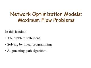
Maximum Flow Problems
Maximum Flow Problems. 204.302 in 2005. A simple network. Note that the nodes in this graph have specific labels for the source and the sink nodes. Capacities and costs. When modelling we usually will have constraints or costs associated with particular edges on the network.


Maximum Flow Problems
E N D
Presentation Transcript
Maximum Flow Problems 204.302 in 2005
A simple network • Note that the nodes in this graph have specific labels for the source and the sink nodes.
Capacities and costs • When modelling we usually will have constraints or costs associated with particular edges on the network. • It is these considerations that determine the amount of flow along a particular edge – denoted xij • Nodes usually get numbered, making the definition of edges and their costs or capacities easier. • For example 0 6 xij6 uij. • Note that xij=-xji if an edge is undirected. • The cost of each direction is not necessarily the same in all contexts, meaning that a pair of directed edges is easier to work with.
What is a max flow problem? As the name suggests, we want to maximize the flow in the network. We give the label “source” to the node that represents the ultimate beginning of the network, and “sink” to the ultimate destination of all product flowing in the network. We will look at an algorithm for finding the maximum flow of the network from source to sink, and A means of determining an upper bound for the maximum flow of the network.
The Ford-Fulkerson algorithm This algorithm finds paths from the source to the sink that can have an increase in its flow. The flow along that path is then adjusted and a new path is sought. Let’s follow a simple example using the network given previously and the table of capacities in the notes.
Finding an augmenting path Obviously any augmenting path must start at the source node. At the first iteration we can “label” both A and B from the source node, and given the current flow is zero, we can label every node in the network. Let’s just take the simple path s-A-D-t for starters. What is the maximum amount this path can be increased while keeping the solution feasible?
A second augmenting flow You should probably mark the reduction in available flow along the edges in the path just augmented. This will then (slightly) limit the options for an augmenting path. The simplest path to choose at the second iteration is s-B-E-t. Check its maximum possible increase is 20.
Third iteration The path s-A-B-E-t could now be augmented. Note that this uses an undirected edge between A and B. After increasing the flow along this path by 10 units, you could draw a reduced network. It appears in the notes as Figure 4. It is a little easier to find the next augmenting path with a reduced network without the clutter of your working. You could choose to augment the path s-A-C-D-t now by the allowable 5 units.
The optimal solution found The optimal solution has been found as there is no possible means of getting any product anywhere from the source node. This leads to the minimum cut maximum flow theorem. Finding a set of edges that split the source and the sink into two disconnected subnetworks means that the max flow has been obtained. This works under certain conditions and must be expanded to allow for all conditions.
Min Cut Max Flow A cut set is a set of edges that if removed from the network leave two disconnected subnetworks having the source cut off from the sink. Finding the cut set that has the least capacity from the source’s subnetwork to the sink’s subnetwork provides an upper bound on the maximum flow of the network. You must look out for the direction of the edges in the cut set. If your current network flow is equal to the capacity of the cut set, you have the optimal solution.