Maximum Flow
Learn about maximum flow concepts in network graphs, capacity constraints, flow conservation, and determining maximum material flow rates from the source to the sink.


Maximum Flow
E N D
Presentation Transcript
Maximum Flow Chapter 26
Flow Concepts • Source vertex s • where material is produced • Sink vertex t • where material is consumed • For all other vertices – what goes in must go out • Flow conservation • Goal: determine maximum rate of material flow from source to sink
Introduction - network Representation Example: oil pipeline Flow network: directed graph G=(V,E) v3 v3 v1 v1 S S t t source v2 v4 v2 v4 sink
Introduction – max-flow problem Representation Example: oil pipeline Flow network: directed graph G=(V,E) v3 v3 v1 v1 S S t t source v2 v4 v2 v4 sink Informal definition of the max-flow problem: What is the greatest rate at which material can be shipped from the source to the sink without violating any capacity contraints?
Introduction - capacity 3 v3 v1 6 8 3 S t 3 6 8 v2 v4 6 c(u,v)=12 6 c(u,v)=6 u u v v Representation Example: oil pipeline Flow network: directed graph G=(V,E) v3 v1 S t v2 v4 12 Big pipe Small pipe
Introduction - capacity Representation Example: oil pipeline Flow network: directed graph G=(V,E) 3 v3 v3 v1 v1 6 8 3 S S t t 3 6 8 v2 v4 v2 v4 6 If (u,v) E c(u,v) = 0 6 v2 v4 0 0 v4 v3 0
Introduction – flow 3 v3 v1 6 8 3 S t 3 6 8 v2 v4 6 f(u,v)=6 f(u,v)=6 u u v v Representation Example: oil pipeline Flow network: directed graph G=(V,E) v3 v1 S t v2 v4 6/12 Flow below capacity 6/6 Maximum flow
Introduction – flow 3 v3 v1 6 8 3 S t 3 6 8 v2 v4 6 Representation Example: oil pipeline Flow network: directed graph G=(V,E) v3 v1 S t v2 v4
Introduction – flow 3 v3 v1 6 8 3 S t 3 6/6 6/8 v2 v4 6/6 Representation Example: oil pipeline Flow network: directed graph G=(V,E) v3 v1 S t v2 v4
Introduction – flow 3 v3 v1 6 8 3 S t 3 6/6 6/8 v2 v4 6/6 Representation Example: oil pipeline Flow network: directed graph G=(V,E) v3 v1 S t v2 v4
Introduction – flow 3/3 v3 v1 3/6 3/8 3 S t 3 6/6 6/8 v2 v4 6/6 Representation Example: oil pipeline Flow network: directed graph G=(V,E) v3 v1 S t v2 v4
Introduction – flow 3/3 v3 v1 3/6 3/8 3 S t 3 6/6 6/8 v2 v4 6/6 Representation Example: oil pipeline Flow network: directed graph G=(V,E) v3 v1 S t v2 v4
Introduction – flow 3/3 v3 v1 3/6 5/8 2/3 S t 3 6/6 8/8 v2 v4 6/6 Representation Example: oil pipeline Flow network: directed graph G=(V,E) v3 v1 S t v2 v4
Introduction – cancellation 3/3 v3 v1 3/6 5/8 2/3 S t 3 6/6 8/8 v2 v4 6/6 Representation Example: oil pipeline Flow network: directed graph G=(V,E) v3 v1 S t v2 v4
Introduction – cancellation 3/3 v3 v1 4/6 6/8 3/3 S t 1/3 6/6 8/8 v2 v4 5/6 Representation Example: oil pipeline Flow network: directed graph G=(V,E) v3 v1 S t v2 v4 u u u u 8/10 3/4 5/10 4 10 4 8/10 4 v v v v
Maximum Flow Problem Given: Directed graph G=(V, E), Supply (source) node O,demand (sink) node T Capacity function u: E R . Goal: Given the arc capacities, send as much flow as possible from supply node O to demand node T through the network. Example: A 4 4 6 B O D 5 5 T 4 4 5 C
Towards the Augmenting Path Algorithm Idea: Find a path from the sourceto the sink, and use it to send as much flow as possible. In our example, 5 units of flow can be sent through the path O B D T ; Then use the path O C T to send 4 units of flow. The total flow is 5 + 4 = 9 at this point. Can we send more? A 4 4 5 5 B 5 O D 5 6 T 4 5 4 4 4 C 5
Towards the Augmenting Path Algorithm If we redirect 1 unit of flow from path O B D T to path O B C T, then the freed capacity of arc D T could be used to send 1 more unit of flow through path O A D T, making the total flow equal to 9+1=10 . To realize the idea of redirecting the flow in a systematic way, we need the concept of residual capacities. A 1 1 4 4 4 5 5 4 B 5 O D 5 6 T 4 5 4 4 1 5 4 C 5
Residual Network The network given by the undirected arcs and residual capacities is called residual network. In our example, the residual network before sending any flow: Note that the sum of the residual capacities on both ends of an arc is equal to the original capacity of the arc. How to increase the flow in the network based on the values of residual capacities? A 0 4 4 0 5 0 6 B 0 O D 5 0 4 4 T 0 0 0 5 C
Residual capacities Suppose we have an arc with capacity 6 and current flow 5: Then there is a residual capacity of 6-5=1 for any additional flow through B D . On the other hand, at most 5 units of flow can be sent back from D to B, i.e., 5 units of previously assigned flow can be canceled. In that sense, 5 can be considered as the residual capacity of the reverse arc D B . To record the residual capacities in the network, we will replace the original directed arcs with undirected arcs: 5 D B 6 5 1 B The number at B is the residual capacity of BD; the number at Dis the residual capacity of DB. D
Augmenting paths An augmenting path is a directed path from the source to the sink in the residual network such that every arc on this path has positive residual capacity. The minimum of these residual capacities is called the residual capacity of the augmenting path. This is the amount that can be feasibly added to the entire path. The flow in the network can be increased by finding an augmenting path and sending flow through it.
Updating the residual network by sending flow through augmenting paths Continuing with the example, Iteration 1: O B D T is an augmenting path with residual capacity 5 = min{5, 6, 5}. After sending 5 units of flow through the path O B D T, the new residual network is: 5 0 6 0 5 0 A 0 5 1 B 5 O D 0 5 T C 0 4 4 0 4 4 0 0 0 5
Updating the residual network by sending flow through augmenting paths Iteration 2: O C T is an augmenting path with residual capacity 4 = min{4, 5}. After sending 4 units of flow through the path O C T, the new residual network is: 0 A 4 4 1 B O D 4 T 0 0 5 C 0 4 4 0 0 5 1 5 0 5 4 0
Updating the residual network by sending flow through augmenting paths Iteration 3: O A D B C T is an augmenting path with residual capacity 1 = min{4, 4, 5, 4, 1}. After sending 1 units of flow through the path O A D B C T , the new residual network is: A 1 0 3 4 3 4 1 0 2 1 B 5 4 O D 4 3 T 5 4 0 1 0 1 C 0 5 0 5 0 4
Terminating the Algorithm:Returning an Optimal Flow There are no augmenting paths in the last residual network. So the flow from the source to the sink cannot be increased further, and the current flow is optimal. Thus, the current residual network is optimal. The optimal flow on each directed arc of the original network is the residual capacity of its reverse arc: flow(OA)=1, flow(OB)=5, flow(OC)=4, flow(AD)=1, flow(BD)=4, flow(BC)=1, flow(DT)=5, flow(CT)=5. The amount of maximum flow through the network is 5 + 4 + 1 = 10 (the sum of path flows of all iterations).
Flow properties Flow network G = (V,E) 12/12 v3 v1 Note: by skew symmetry f (v3,v1) = - 12 11/16 15/20 10 1/4 7/7 S t 4/9 4/4 8/13 v2 v4 11/14
Net flow and value of a flow u u f(u,v) = 5 f(v,u) = -5 8/10 3/4 5/10 4 v v 3/3 v3 v1 4/6 6/8 3/3 S t 1/3 6/6 8/8 v2 v4 5/6
The max-flow problem Informal definition of the max-flow problem: What is the greatest rate at which material can be shipped from the source to the sink without violating any capacity contraints? Formal definition of the max-flow problem: The max-flow problem is to find a valid flow for a given weighted directed graph G, that has the maximum value over all valid flows.
The Ford-Fulkerson methoda way how to find the max-flow This method contains 3 important ideas: 1) residual networks 2) augmenting paths 3) cuts of flow networks
Ford-Fulkerson – pseudo code 1 initialize flow f to 0 2 while there exits an augmenting path p 3do augment flow f along p 4 return f
Ford Fulkerson – residual networks 5 11 5 8 cf(u,v) = c(u,v) – f(u,v) The residual network Gf of a given flow network G with a valid flow f consists of the same vertices v V as in G which are linked with residual edges (u,v) Ef that can admit more strictly positive net flow. The residual capacity cf represents the weight of each edge Ef and is the amount of additional net flow f(u,v) before exceeding the capacity c(u,v) Flow network G = (V,E) residual network Gf = (V,Ef) 12/12 v3 v3 v1 v1 11/16 15/20 10 1/4 7/7 S t S t 4/9 4/4 8/13 v2 v4 v2 v4 11/14
Ford Fulkerson – residual networks cf(u,v) = c(u,v) – f(u,v) The residual network Gf of a given flow network G with a valid flow f consists of the same vertices v V as in G which are linked with residual edges (u,v) Ef that can admit more strictly positive net flow. The residual capacity cf represents the weight of each edge Ef and is the amount of additional net flow f(u,v) before exceeding the capacity c(u,v) Flow network G = (V,E) residual network Gf = (V,Ef) 12 12/12 v3 v3 v1 v1 5 5 11/16 15/20 4 11 10 1/4 11 7/7 7 15 3 S t S t 4/9 5 5 4/4 4 3 8/13 8 v2 v4 v2 v4 11/14 11
Ford Fulkerson – augmenting paths Definition: An augmenting path p is a simple (free of any cycle) path from s to t in the residual network Gf Residual capacity of p cf(p) = min{cf (u,v): (u,v) is on p} Flow network G = (V,E) residual network Gf = (V,Ef) 12 12/12 v3 v3 v1 v1 5 5 11/16 15/20 4 11 10 1/4 11 7/7 7 15 3 S t S t 4/9 5 5 4/4 4 3 8/13 8 v2 v4 v2 v4 11/14 11
Ford Fulkerson – augmenting paths Definition: An augmenting path p is a simple (free of any cycle) path from s to t in the residual network Gf Residual capacity of p cf(p) = min{cf (u,v): (u,v) is on p} Flow network G = (V,E) residual network Gf = (V,Ef) 12 12/12 v3 v3 v1 v1 5 5 11/16 15/20 4 11 10 1/4 11 7/7 7 15 3 S t S t 4/9 5 5 4/4 4 3 8/13 8 v2 v4 v2 v4 11/14 11 Augmenting path
Ford Fulkerson – augmenting paths We define a flow: fp: V x V R such as: cf(p) if (u,v) is on p fp(u,v) = - cf(p) if (v,u) is on p 0 otherwise Flow network G = (V,E) residual network Gf = (V,Ef) 12 12/12 v3 v3 v1 v1 5 5 11/16 15/20 4 11 10 1/4 11 7/7 7 15 3 S t S t 4/9 5 5 4/4 4 3 8/13 8 v2 v4 v2 v4 11/14 11
Ford Fulkerson – augmenting paths cf(p) if (u,v) is on p fp(u,v) = - cf(p) if (v,u) is on p 0 otherwise We define a flow: fp: V x V R such as: Flow network G = (V,E) residual network Gf = (V,Ef) 12 12/12 v3 v3 v1 v1 5 4/5 11/16 15/20 4/4 11 10 1/4 11 7/7 7 -4/15 3 S t S t 4/9 -4/5 4/5 4/4 4 3 8/13 -4/8 v2 v4 v2 v4 11/14 11 Our virtual flow fp along the augmenting path p in Gf
Ford Fulkerson – augmenting paths cf(p) if (u,v) is on p fp(u,v) = - cf(p) if (v,u) is on p 0 otherwise We define a flow: fp: V x V R such as: Flow network G = (V,E) residual network Gf = (V,Ef) 12 12/12 v3 v3 v1 v1 5 4/5 11/16 15/20 4/4 11 10 1/4 11 7/7 7 -4/15 3 S t S t 4/9 -4/5 4/5 4/4 4 3 8/13 -4/8 v2 v4 v2 v4 11/14 11 Our virtual flow fp along the augmenting path p in Gf
Ford Fulkerson – augmenting the flow cf(p) if (u,v) is on p fp(u,v) = - cf(p) if (v,u) is on p 0 otherwise We define a flow: fp: V x V R such as: Flow network G = (V,E) residual network Gf = (V,Ef) 12 12/12 v3 v3 v1 v1 5 4/5 11/16 19/20 4/4 11 10 1/4 11 7/7 7 15 3 S t S t 0/9 5 4/5 4/4 4 3 12/13 8 v2 v4 v2 v4 11/14 11 New flow: f´: V x V R : f´=f + fp Our virtual flow fp along the augmenting path p in Gf
Ford Fulkerson – new valid flowproof of capacity constraint cf(p) if (u,v) is on p fp(u,v) = - cf(p) if (v,u) is on p 0 otherwise Lemma: f´ : V x V R : f´ = f + fp in G cf(p) = min{cf (u,v): (u,v) is on p} Capacity constraint: For all u,v V, we require f(u,v) < c(u,v) cf(u,v) = c(u,v) – f(u,v) Proof: fp (u ,v) < cf (u ,v) = c (u ,v) – f (u ,v) (f + fp) (u ,v) = f (u ,v) + fp (u ,v) < c (u ,v)
The Ford-Fulkerson method Ford-Fulkerson(G,s,t) 1 for each edge (u,v) in G.E do 2 f(u,v) ¬ f(v,u) ¬ 0 3 while there exists a path p from s to t in residual network Gfdo 4 cf = min{cf(u,v): (u,v) is in p} 5 for each edge (u,v) in p do 6 f(u,v) ¬ f(u,v) + cf 7 f(v,u)¬-f(u,v) 8 return f The algorithms based on this method differ in how they choose p in step 3. If chosen poorly the algorithm might not terminate.
Execution of Ford-Fulkerson (1) Left Side = Residual Graph Right Side = Augmented Flow
Execution of Ford-Fulkerson (2) Left Side = Residual Graph Right Side = Augmented Flow
Cuts • Does the method find the minimum flow? • Yes, if we get to the point where the residual graph has no path from s to t • A cut is a partition of V into S and T = V – S, such that s S and t T • The net flow (f(S,T)) through the cut is the sum of flows f(u,v), where s S and t T • Includes negative flows back from T to S • The capacity (c(S,T)) of the cut is the sum of capacities c(u,v), where s S and t T • The sum of positive capacities • Minimum cut – a cut with the smallest capacity of all cuts. |f|= f(S,T) i.e. the value of a max flow is equal to the capacity of a min cut. 8/13 a b 10/15 13/19 10 t s 5/5 9 2/4 6/14 8/11 3/3 c d Cut capacity = 24 Min Cut capacity = 21
Max Flow / Min Cut Theorem • Since |f| c(S,T) for all cuts of (S,T) then if |f| = c(S,T) then c(S,T) must be the min cut of G • This implies that f is a maximum flow of G • This implies that the residual network Gf contains no augmenting paths. • If there were augmenting paths this would contradict that we found the maximum flow of G • 1231 … and from 23 we have that the Ford Fulkerson method finds the maximum flow if the residual graph has no augmenting paths.
Worst Case Running Time • Assuming integer flow • Each augmentation increases the value of the flow by some positive amount. • Augmentation can be done in O(E). • Total worst-case running time O(E|f*|), where f* is the max-flow found by the algorithm. • Example of worst case: Augmenting path of 1 Resulting Residual Network Resulting Residual Network
Application – Bipartite Matching • Example – given a community with n men and m women • Assume we have a way to determine which couples (man/woman) are compatible for marriage • E.g. (Joe, Susan) or (Fred, Susan) but not (Frank, Susan) • Problem: Maximize the number of marriages • No polygamy allowed • Can solve this problem by creating a flow network out of a bipartite graph
Bipartite Graph • A bipartite graph is an undirected graph G=(V,E) in which V can be partitioned into two sets V1 and V2 such that (u,v) E implies either u V1 and v V12 or vice versa. • That is, all edges go between the two sets V1 and V2 and not within V1 and V2.
Model for Matching Problem • Men on leftmost set, women on rightmost set, edges if they are compatible A A A X X X B B B Y Y Y C C C Z Z Z D D D Men Women Optimal matching A matching
Solution Using Max Flow • Add a supersouce, supersink, make each undirected edge directed with a flow of 1 A A X X B B t Y s Y C C Z Z D D Since the input is 1, flow conservation prevents multiple matchings