Model of the theoretical gravity
210 likes | 392 Vues
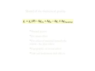
Model of the theoretical gravity. Normal gravity Elevation effect The effect of material beneath the station - the plate effect Topographic or terrain effect Tide and Instrument drift effects. More on the terrain correction -.

Model of the theoretical gravity
E N D
Presentation Transcript
Model of the theoretical gravity • Normal gravity • Elevation effect • The effect of material beneath the station - the plate effect • Topographic or terrain effect • Tide and Instrument drift effects
More on the terrain correction - In dealing with the derivation of the Bouguer plate effect you may have realized that the trick to integration was in how one defined the volume element. This remains true in computing the acceleration of a ring. The approach to the terrain correction rests on the analytical expression derived for the acceleration due to gravity of the ring - in particular a given sector of the ring. We start by deriving the acceleration over a disk with 0 inner radius and outer radius R0. Our starting point should be familiar by now -
and assuming that we have constant density throughout the disk
Consider the following- • What happens when R0 goes to ? g=2G (h) where h is just the thickness of the plate and could be z or just z using the notation of the text. This is just the Bouguer plate correction.
g drift Drift density contrast t drift thickness This is just the plate correction. At infinity the effect of ring and plate are the same.
The foregoing approach represents another way to derive the plate correction - and also to determine the effect of a ring.
Remember we want to approximate topographic features by ring sectors because it’s easy to compute the effect of a ring sector on the observed gravity.
The Anomaly Now that we’ve described all the corrections and gained some experience and familiarity with their computation, let’s consider the concept of the gravity anomaly. What is a gravity anomaly? In general an anomaly is considered to be the difference between what you actually have and what you thought you’d get. In gravity applications you make an observation of the acceleration due to gravity (gobs) at some point and you also calculate or make a prediction about what the gravity should be at that point (gt). The prediction assumes you have a homogeneous earth - homogeneous in the sense that the earth can consist of concentric shells of differing density, but that within each shell there are no density contrasts. Similar assumptions are made in the computation of the plate and topographic effects. gt then, in most cases, is an imperfect estimate of acceleration. Some anomaly exists. ganom= gobs - gt
This is a simple definition, but there are several different types of anomalies, which depend on the degree to which the theoretical gravity has been estimated. For example, in an area relatively close to sea-level we might only include the elevation effect in the computation of gt. This would also be standard practice in ocean surveys. In general tide and drift effects are always included. In this case, the anomaly (ganom) is referred to as the free-air anomaly (FAA).
When only the elevation and plate effects are included in the computation of theoretical gravity, the anomaly is referred to as the simple Bouguer anomaly or just the Bouguer anomaly. The combined corrections are often referred to as the elevation correction.
When all the terms, including the terrain effect are included in the computation of the gravity anomaly, the resultant anomaly is referred to as the complete Bouguer anomaly or the terrain corrected Bouguer anomaly (gTBA).
In this form - The different terms in the theoretical gravity are referred to as corrections. Thus - gFA is referred to as the free-air correction gB is referred to as the Bouguer plate correction gT is referred to as the terrain correction, and gTide and Drift is referred to as the tide and drift correction
Long wavelength features are often referred to as the regional field. The regional variations are highlighted here in green. The residual is the difference between the anomaly (whichever it is) and the regional field.
Separation of Regional & Residual Examine the map at right. Note the regional and residual (or local) variations in the gravity field through the area. The graphical separation method involves drawing lines through the data that follow the regional trend. The green lines at right extend through the residual feature and reveal what would be the gradual drop in the anomaly across the area if the local feature were not present.
The residual anomaly is identified by marking the intersections of the extended regional field with the actual anomaly and labeling them with the value of the actual anomaly relative to the extended regional field. -1 -0.5 -0.5 After labeling all intersections with the relative (or residual ) values, you can contour these values to obtain a map of the residual feature.
Geology 252 • Environmental and Exploration Geophysics I • In-Class Exercise - Determining residual acceleration • Use the graphical construction approach and estimate the residual anomaly superimposed on the regional gravity gradient. • What is the maximum value of the residual anomaly? • What is the minimum value of the residual anomaly? • Is the anomaly positive or negative? Bring your results to lab
Non-Uniqueness Note that a particular anomaly, such as that shown below, could be attributed to a variety of different density distributions. gravity anomaly Note also, however, that there is a certain maximum depth beneath which this anomaly cannot have its origins. Nettleton, 1971