Download
1 / 31
320 likes | 353 Vues
EECS 122: QoS and Packet Scheduling: Token-Bucket, WFQ, Hierarchical Link Sharing. Computer Science Division Department of Electrical Engineering and Computer Sciences University of California, Berkeley Berkeley, CA 94720-1776. Quality of Service (QoS). IP provides only best effort service

E N D
EECS 122: QoS and Packet Scheduling: Token-Bucket, WFQ, Hierarchical Link Sharing Computer Science Division Department of Electrical Engineering and Computer Sciences University of California, Berkeley Berkeley, CA 94720-1776
Quality of Service (QoS) • IP provides only best effort service • Many applications want better services • IP telephony • Video teleconferencing • …. • Design a network that provides better than best-effort service • Basic service parameters • Delay • Bandwidth • Loss rate
QoS Service • A contract between end-hosts and the network • End-host specify • Traffic characteristics (e.g., send no more than 100 Kbps) • Service requirements (e.g., delay < 50ms, loss < 0.1%) • Network performs: • Admission control: check whether it can grant end-host’s wish • Reserve resources for the traffic sent by end-host • Schedule packets to make sure that end-host’s requirements are met • If end-host violates the contract (e.g., sends more traffic than it said) all bets are off!
QoS Granularity • Flow/Aggregate identified by a subset of following fields in the packet header • source/destination IP address (32 bits) • source/destination port number (16 bits) • protocol type (8 bits) • type of service (8 bits) • Examples: • All packets from machine A to machine B • All packets from Berkeley • All packets between Berkeley and MIT • All TCP packets from EECS-Berkeley
Token Bucket • A simple traffic model used to: • Enforce traffic sent by a sender (e.g., cable modem) • Characterize the traffic sent by a sender
Token Bucket • Parameters • r – average rate, i.e., rate at which tokens fill the bucket • b – bucket depth • R – maximum link capacity or peak rate (optional parameter) • A bit is transmitted only when there is an available token Maximum # of bits sent r bps bits slope r b*R/(R-r) b bits slope R <= R bps time regulator
(b) (a) 3Kb 2.2Kb T = 2ms : packet transmitted b = 3Kb – 1Kb + 2ms*100Kbps = 2.2Kb T = 0 : 1Kb packet arrives (c) (d) (e) 3Kb 2.4Kb 0.6Kb T = 4ms : 3Kb packet arrives T = 10ms : packet needs to wait until enough tokens are in the bucket! T = 16ms : packet transmitted Traffic Enforcement: Example • r = 100 Kbps; b = 3 Kb; R = 500 Kbps
Source Traffic Characterization: Arrival Curve • Arrival curve – maximum amount of bits transmitted during an interval of time Δt • Use token bucket to bound the arrival curve bps bits Arrival curve Δt time
(R=2,b=1,r=1) Arrival Curve: Example • Arrival curve – maximum amount of bits transmitted during an interval of time Δt • Use token bucket to bound the arrival curve Arrival curve bits 4 bps 3 2 2 1 1 Δt 0 1 2 3 4 5 1 2 3 4 5 time
D Ba QoS Guarantees: Per-hop Reservation • End-host: specify • the arrival rate characterized by token-bucket with parameters (b,r,R) • the maximum maximum admissible delay D, no losses • Router: allocate bandwidth ra and buffer space Ba such that • no packet is dropped • no packet experiences a delay larger than D slope ra slope r bits Arrival curve b*R/(R-r) R
Packet Scheduling • Decide when and what packet to send on output link • Make sure that the flow gets the allocated bandwidth • Usually implemented at output interface of a router flow 1 Classifier flow 2 Scheduler 1 2 flow n Buffer management
Packet Scheduling: Example • Make sure that at any time the flow receives at least the allocated rate ra • The canonical example of such scheduler: Weighted Fair Queueing (WFQ)
Weighted Fair Queueing (WFQ) • Implements max-min fairness: each flow receives min(ri, f) , where • ri– flow arrival rate • f – link fair rate (see next slide) • Weighted Fair Queueing (WFQ) – associate a weight with each flow
Fair Rate Computation: Example 1 • If link congested, compute f such that f = 4: min(8, 4) = 4 min(6, 4) = 4 min(2, 4) = 2 8 10 4 6 4 2 2
Flow i is guaranteed to be allocated a rate >= wi*C/(Σk wk) If Σk wk <= C, flow i is guaranteed to be allocated a rate >= wi Fair Rate Computation: Example 2 • Associate a weight wiwith each flow i • If link congested, compute f such that f = 2: min(8, 2*3) = 6 min(6, 2*1) = 2 min(2, 2*1) = 2 8 (w1 = 3) 10 4 6 (w2 = 1) 4 2 2 (w3 = 1)
Fluid Flow System • Flows can be served one bit at a time • WFQ can be implemented using bit-by-bit weighted round robin • During each round from each flow that has data to send, send a number of bits equal to the flow’s weight
transmission time 3 4 5 1 2 C 1 2 3 4 5 6 Fluid Flow System: Example 1 Flow 1 (w1 = 1) 100 Kbps Flow 2 (w2 = 1) Flow 1 (arrival traffic) 1 2 4 5 3 time Flow 2 (arrival traffic) 1 2 3 4 5 6 time Service in fluid flow system time (ms) 0 10 20 30 40 50 60 70 80 Area (C x transmission_time) = packet size
Fluid Flow System: Example 2 link • Red flow has sends packets between time 0 and 10 • Backlogged flow flow’s queue not empty • Other flows send packets continuously • All packets have the same size flows weights 5 1 1 1 1 1 0 2 4 6 8 10 15
Implementation In Packet System • Packet (Real) system: packet transmission cannot be preempted. • Solution: serve packets in the order in which they would have finished being transmitted in the fluid flow system
Select the first packet that finishes in the fluid flow system 1 2 1 3 2 3 4 4 5 5 6 Packet System: Example 1 Service in fluid flow system 3 4 5 1 2 1 2 3 4 5 6 time (ms) Packet system time
Select the first packet that finishes in the fluid flow system Packet System: Example 2 Service in fluid flow system 0 2 4 6 8 10 Packet system 0 2 4 6 8 10
Implementation Challenge • Need to compute the finish time of a packet in the fluid flow system… • … but the finish time may change as new packets arrive! • Need to update the finish times of all packets that are in service in the fluid flow system when a new packet arrives • But this is very expensive; a high speed router may need to handle hundred of thousands of flows!
Finish times computed at time 0 time 0 1 2 3 Finish times re-computed at time ε time 0 1 2 3 4 Example • Four flows, each with weight 1 Flow 1 time Flow 2 time Flow 3 time Flow 4 time ε
Solution: Virtual Time • Key Observation: while the finish times of packets may change when a new packet arrives, the order in which packets finish doesn’t! • Only the order is important for scheduling • Solution: instead of the packet finish time maintain the number of rounds needed to send the remaining bits of the packet (virtual finishing time) • Virtual finishing time doesn’t change when the packet arrives • System virtual time – index of the round in the bit-by-bit round robin scheme
System Virtual Time: V(t) • Measure service, instead of time • V(t) slope – normalized rate at which every backlogged flow receives service in the fluid flow system • C – link capacity • N(t) – total weight of backlogged flows in fluid flow system at time t V(t) time
System Virtual Time (V(t)): Example 1 • V(t) increases inversely proportionally to the sum of the weights of the backlogged flows Flow 1 (w1 = 1) time Flow 2 (w2 = 1) time 3 4 5 1 2 1 2 3 4 5 6 V(t) C/2 C
System Virtual Time: Example w1 = 4 w2 = 1 w3 =1 w4 =1 w5 =1 V(t) C/4 C/8 C/4 0 4 8 12 16
Fair Queueing Implementation • Define • - virtual finishing time of packet k of flow i • - arrival time of packet k of flow i • - length of packet k of flow i • wi – weight of flow i • The finishing time of packet k+1 of flow i is / wi
Properties of WFQ • Guarantee that any packet is transmitted within packet_lengt/link_capacity of its transmission time in the fluid flow system • Can be used to provide guaranteed services • Achieve max-min fair allocation • Can be used to protect well-behaved flows against malicious flows
Hierarchical Link Sharing 155 Mbps Link 55 Mbps 100 Mbps Provider 1 Provider 2 50 Mbps 50 Mbps Berkeley Stanford. • Resource contention/sharing at different levels • Resource management policies should be set at different levels, by different entities • Resource owner • Service providers • Organizations • Applications 20 Mbps 10 Mbps Math Campus EECS seminar video seminar audio WEB
Packet Approximation of H-WFQ • Idea 1 • Select packet finishing first in H-WFQ assuming there are no future arrivals • Problem: • Finish order in system dependent on future arrivals • Virtual time implementation won’t work • Idea 2 • Use a hierarchy of WFQ to approximate H-WFQ Fluid Flow H-WFQ Packetized H-WFQ 10 10 WFQ WFQ 6 4 6 4 WFQ WFQ WFQ WFQ 1 1 3 3 2 2 WFQ WFQ WFQ WFQ WFQ WFQ