Download
1 / 52
520 likes | 627 Vues
This summary explores the fundamentals of demand and price dynamics, including the demand curve, market equilibrium, price elasticity, and profit maximization strategies. It delves into concepts such as the market mechanism, price surpluses, elasticity of demand, and cost categories. The text also covers the learning curve, breakeven analysis, and the allocation of costs for strategic decision-making. In addition, it discusses the principles of profit maximization and price discrimination, highlighting examples and strategies for optimizing revenues in varying market conditions.

E N D
Demand curve – shows how D depends on P. Also depends on income. Price Demand curve shifts out as income Rises. Quantity demanded or supplied
S The curves intersect at equilibrium, or market- clearing, price. At P0the quantity supplied is equal to the quantity demanded at Q0 . P0 D Q0 The Market Mechanism Price ($ per unit) Quantity
Price ($ per unit) S Surplus P1 Assume the price is P1 , then: 1) Qs : Q1 > Qd : Q2 2) Excess supply is Q1:Q2. 3) Producers lower price. 4) Quantity supplied decreases and quantity demanded increases. 5) Equilibrium at P2Q3 P2 D Quantity Q1 Q3 Q2 The Market Mechanism
Measures responsiveness of demand to price. Defined as E = (dQ/Q)/(dP/P) = (dQ/dP)*(P/Q) Why is it defined in proportional terms? - Unit free. - Scale sensitive. A negative number. Price elasticity of demand:
Critical in understanding oil market, energy markets, metal markets Responding to a price movement takes time - possibly many years Long-run elasticity measures total response Short-run elasticity measures immediate response Short-run vs. long-run elasticities
Summary on demand: • How demand depends on prices and income. • How the time period (s-r vs l-r) affects response to prices and incomes. • How D and S interact to determine prices. • How revenue varies with output.
The Learning Curve Hours of labor per machine lot • The horizontal axis measures the cumulative number of hours of machine tools the firm has produced • The vertical axis measures the number of hours of labor needed to produce each lot. 10 8 6 4 2 0 10 20 30 40 50
Breakeven: • Occurs at the output level at which total cost equals total revenue. • Let P(N) be the price at which N units can be sold. Then breakeven means: P(N) . N = FC + VC(N)
Study the elasticity of profits with respect to output Q. Let output change from Q to Q + Q, and profits from to + Intuition - must be greater, the greater are fixed costs. Leverage
Table 4Reconfigured Income Statement for Product A Using a Variable Budget Format (1000s) Sales (40 million lbs. @ 50 cents/lb) $20,000 less: Variable Costs: Materials 8,000 Direct labour 2,000 Manufacturing overhead 1,000 Sales Commissions 1.000 Total Variable Costs 12,000 Variable Margin (Profit Contribution) 8,000 less: Fixed Costs: Advertising 800 Promotion 200 Field Sales 2,200 Product Management 50 Marketing Management 300 Product Development 300 Marketing Research 150 Manufacturing Overhead 1,200 General and Administrative 1,400 Total Fixed Costs 6,600 Net Profit Before Taxes 1,400
Summary on Costs: • Identify which cost are relevant to a decision. • Distinguish fixed and variable costs and use this to determine impact of output change on profits. • Understand allocation of overhead costs. • Determine when to shut down in short and long runs. • Analyze breakeven.
C $ t' R 400 300 c t 200 150 Profits 100 50 c 0 5 10 15 20 Quantity Example of Profit Maximization • Observations • Slope of rr’ = slope cc’ and they are parallel at 10 units • Profits are maximized at 10 units • P = $30, Q = 10, TR = P x Q = $300 • AC = $15, Q = 10, TC = AC x Q = 150 • Profit = TR - TC • $150 = $300 - $150
$/Q 40 MC 30 AC Profit 20 AR 15 MR 10 0 5 10 15 20 Quantity Example of Profit Maximization • Observations • AC = $15, Q = 10, TC = AC x Q = 150 • Profit = TR = TC = $300 - $150 = $150 or • Profit = (P - AC) x Q = ($30 - $15)(10) = $150
The more elastic is demand, the less the markup. P* MC MC P* AR P*-MC MR AR MR Q* Q* Elasticity of Demand and Price Markup $/Q $/Q Quantity Quantity
1 Ep For maximum profits, MR = MC so P + P = MC Or P - MC = - 1 P Ep
Consumer Surplus • With a downward sloping demand curve, and uniform price for all buyers, some buyers will be paying less than they are willing to pay for the good (for example, the buyers at the top left hand end of the demand curve)
Examples of Price Discrimination • By country – Cars, pharmaceuticals, Reuters. (Becoming more difficult.) • By income level – catalogs (zip code), The Gap, Mexican retail, supermarkets chains by location, Switzerland in food brands, • On line – double click (possible bypass via anonymizer etc.). • No price list – individualized prices.
The Two-Part Tariff • The purchase of some products and services can be separated into two decisions, and therefore, two prices • Decision to enter market and decision about how much to buy
The Two-Part Tariff • Examples 1) Amusement Park • Pay to enter • Pay for rides and food within the park 2) Tennis Club • Pay to join • Pay to play
The Two-Part Tariff • Pricing decision is setting the entry fee (T) and the usage fee (P) • Choosing the trade-off between free-entry and high user charges or high-entry and zero user charges
User price P* is set at MC. Entry price T* is equal to the entire consumer surplus. T* MC P* Two-Part Tariff with a Single Type of Consumer $/Q D Quantity
Bundling • Selling several goods in one bundle • Hardware and software • Software suites • Auto accessories
A & B are individuals described by the amounts they are willing to pay for each good. A will pay $9.25 for the bundle and B, $11.50. To sell 1 and 2 separately and get both customers to buy both, cannot charge more than $3.25 for either good. Gives revenue of 4x$3.25 = $13. Bundling gets $2x$9.25 = $18.50. Selling only to customer willing to pay most gets $6 + $8.25 = $14.25. Selling 1 for $8.25 and 2 for $3.25 gets $8.25 + $6.50 = $14.75.
C1 = MC1 C1 = 20 With positive marginal costs, mixed bundling may be more profitable than pure bundling. A Consumer A, for example, has a reservation price for good 1 that is below marginal cost c1. With mixed bundling, consumer A is induced to buy only good 2, while consumer D is induced to buy only good 1, reducing the firm’s cost. B C C2 = MC2 C2 = 30 D Mixed Versus Pure Bundling r2 100 90 80 70 60 50 40 30 20 10 r1 10 20 30 40 50 60 70 80 90 100
Pricing Cell-Phones A mix of discrimination, bundling and two-part pricing Buy the phone (connection/membership charge) & pay for service - like Polaroid, Gilette. Phones at different price points. Then you have a choice between several two-part tariffs
Typically $40 per month with 400 minutes free and 40c/min additionally or $60 per month with 600 minutes free and 30c/min additionally, etc. Choice of two-part tariffs - intended to price discriminate. Heavy users - willing to pay a lot - will opt for high fixed charge to get the lower per unit price, and vice versa. Different two-part tariffs
Pricing policy • For each market segment try to estimate • Maximum consumption if marginal consumption cost is zero. • Consumer surplus at this consumption level. • Use this surplus as a fixed monthly charge and then have a steep fee for going over the allotted number of minutes.
Key aspects • So selling 400 minutes for $40 is NOT the same as selling each minute at the average price, 40/400 = $0.10. • Selling the 400 minutes together is twice as profitable as selling each minute at $0.10. WHY? • Bundling earlier and later minutes together.
e-con.com How do the principles of managerial economics apply in the internet world? Look at Cost structures Selling information Pricing strategies & auctions Industry Standards.
Information Products Much of what the Internet excels at is providing information Information is expensive to Produce but Cheap to Reproduce So average cost is high but marginal cost is low. Competition may lead prices down to MC
Encyclopedia Britanica 1991: EB sold @ $1,600 1992: Microsoft introduced Encarta (bought rights to Funk & Wagnalls), sold @ $49.95 1995: EB’s sales have halved 1995: EB offers on-line subscription for $120 p.a. or CD for $200
Encyclopedia Britanica 1996: EB lowers cost of sub to $85 1999: EB offers FREE on-line service (www.britanica.com) Key point: costs of producing EB are fixed and sunk. Cost of reproducing - MC- is low, zero on-line. Similar story with Yellow Pages. Long distance?
Selling Information • Reuters, financial analysts are bundling information with something else that makes it possible to charge • Few examples of successful businesses that sell information only – usually sell it bundled with something else
Intellectual Property Rights • Digital distribution of “information” (which includes music, videos, software and book) poses serious challenges to property rights of the owners – MC is zero • Hence legal & economic activity on IPR front. Napster, BMG, peer-to-peer file sharing etc. (Another issue – unbundling disk tracks)
Information Products • Bottom line - • Few good business models for making money from selling information over the internet. Business models still needed for Yahoo et al. (eBay is an exception) • Napster shows clearly the likely impact of internet distribution on pricing of digital information.
Auctions • Auctions facilitate price discrimination • Auction Formats • Traditional English (oral, ascending prices, first or second price) • Dutch auction (descending prices) • Sealed-bid (as in T Bills, oil exploration) • First price • Second price
Auctions Common Value Auction • Winner’s Curse • The winner is worse off than those who did not win • Winner is bidder who estimates value of object to be greatest, and so is likely to be overestimating.
Economies of Adoption: Examples - software for Windows vs. Mac, Palm operating system and third party support for these. Large user base means more third party products. Also third party services such as training. Network Effects of Standards
Network Effects Main issue in these cases - fax, e-mail etc are more useful, the more people use them So once they take off there is positive feedback. Demand creates demand. Economies of adoption.
EBAY • Most successful pure Internet company • No bricks & mortar – low fixed costs, no variable costs • Central function – providing info about buyers to sellers & about sellers to buyers • Providing info is key function of a market – well suited to Internet
EBAY • Note Yahoo & Amazon both ran FREE auctions to enter this market yet still have small shares • EBAY has a good business model as it is clear how they can charge for the info they provide – as broker – unlike Yahoo
AOL • AOL – provides info and Yahoo-like services but charges as ISP, also a clear business model • Also gets advertising revenues
Demand for any one PC makers’ product is elastic whereas Demand for Windows, Office and microprocessors is highly inelastic. Barriers to entering and competing translate into inelastic demand and higher profits. Summary
AMAX case Cost Analysis Fixed & variable Average & Marginal Breakeven Entry/Exit Choice Operating leverage Demand & supply Price & Income elasticities PED & MR Forecasting TV Listing Guide Use of income statements Pricing: MR = MC Markup over MC depends on PED Consumer surplus Discrimination Two-part pricing Bundling NYNEX Airlines Cell phones