Download
1 / 88
880 likes | 1.02k Vues
Investment in Business Cycle Models. Miles Kimball. The Power of Investment in Business Cycle Models. The technology-induced fluctuations in standard Real Business Cycle models are fundamentally investment booms.

E N D
Investment in Business Cycle Models Miles Kimball
The Power of Investment in Business Cycle Models • The technology-induced fluctuations in standard Real Business Cycle models are fundamentally investment booms. • Kimball and Ramnath: “With Realistic Parameters the Basic Real Business Cycle model Acts Like the Solow Growth Model” • Basu, Fernald, Fisher and Kimball: “Sector-Specific Technology Shocks” • Including investment dramatically changes the behavior of sticky-price models. • Barsky, House, and Kimball: “Durable Goods and Sticky-Price Models III. The Neomonetarist Synthesis (Kimball) IV. A catastrophic collapse of investment was a key propagation mechanism for the Great Depression. (Barsky and Kimball)
“With Realistic Parameters the Basic Real Business Cycle Model Acts Like the Solow Growth Model” • To match the lack of strong long-run trend in labor hours, Real Business Cycle models need King-Plosser-Rebelo preferences, engineered to get W=Cv’(N), or equivalently, N=v’-1(W/C). • Technology shocks are permanent. --A priori argument: Useful knowledge not soon forgotten --Direct evidence from “Are Technology Improvements Contractionary?” by Basu, Fernald and Kimball • The elasticity of intertemporal substitution is low. --Consumption Euler equation evidence (Hall) --Hypothetical choice evidence (Kimball, Sahm and Shapiro)
“With Realistic Parameters the Basic Real Business Cycle Model Acts Like the Solow Growth Model” • Given King-Plosser-Rebelo preferences with an elasticity of intertemporal substitution of about 0.3, permanent technology shocks have essentially no effect on I/Y or N. • These two results are linked. Multiply Cv’(N)=W by N/C: Nv’(N) = WN/C = (WN/Y) / (C/Y) = (1-α) / (C/Y). 1-α is labor’s share. Given Cobb-Douglas, N depends only on C/Y (negatively). Note that C/Y = 1-(I/Y)-(G/Y). • Thus, N will increase only if I/Y or G/Y increases: if a tech shock does not induce an investment boom, it does not raise labor hours. • Instead, output and investment go up by the same percentage due to the direct effect of the technology shock, and capital accumulates. (Same as the response of Solow Growth Model to a perm. tech shock)
Sector-Specific Technical Change Susanto Basu Boston College and NBER Jonas Fisher Federal Reserve Bank of Chicago John Fernald Federal Reserve Bank of San Francisco Miles Kimball University of Michigan and NBER Very preliminary
Where does growth originate? • Technical change differs across industries • Recent work has highlighted that the final-use sector in which technical change occurs matters • Greenwood, Hercowitz, Krusell • Use relative price data • We reconsider the evidence • Extending GHK to situations where relative pricesmight not measure technology correctly • Top down versus bottom up
Outline • Motivation: Consumption-technology neutrality • How to think about terms of trade? • Disaggregating: Manipulating the input-output matrix • Comparing bottom-up versus top-down estimates
Consumption Technology Neutrality • Suppose utility is logarithmic • Suppose there is some multiplicative technology A for producing non-durable consumption goods • The stochastic process for consumption-technology A affects only the production of nondurable consumption goods • It does not affect affect labor hours N, investment I, or an index of the resources devoted to producing consumption goods X.
Consider social-planners problem for two-sector growth model, with CRS, identical production technologies
This is Special Case of Following, Simple Social Planner’s Problem Equivalent problem:
Comments • Because ln(A) is an additively-separable term, any stochastic process for A has no effect on the optimal decision rules for N, X and I. • There is a weaker, but still important result for the more general King-Plosser-Rebelo case: • anticipated movements in Aact like changes in the utility discount rate • unanticipated movements in A have no effect on the optimal decision rules for N, X and I.
King-Plosser-Rebelo Utility with EIS < 1 (γ>1) Equivalent problem:
An Example: Mean-Reverting Consumption Technology • If A follows an AR(1) process, then At /A0 < 1 after an increase in A above the steady-state level at time zero. • This makes (At /A0)1-γ> 1, which has the same effect as if the discount factor β were larger. • Higher β (greater patience) would lead to an increase in investment I, an increase in labor hours N, and a reduction in the resources devoted to consumption X. • Thus, At /A0 < 1 leads to an increase in investment I, an increase in labor hours N, and a reduction in the resources devoted to consumption X. • However, C=AX may increase even though X decreases.
Empirical Implications: Standard RBC Parameters • With the standard parametrizations of the utility function consumption technology shocks will have very different effects from investment technology shocks. • consumption technology shocks have no effect on labor hours or investment. • investment technology shocks have the same effect on labor hours and investment as pervasive technology shocks. • therefore, like pervasive technology shocks in standard RBC models, investment technology shocks should have a large effect on labor hours and investment.
Empirical Implications: Low EIS and Permanent Tech Shocks • With permanent technology shocks and King-Plosser-Rebelo utility and relatively low elasticity of intertemporal substitution (≈ 0.3), investment technology shocks also have very little immediate effects on labor hours, though they do raise investment in a way that consumption technology shocks do not.
A More General Question • Example of consumption technology neutrality raises possibility that shocks to different final sectors have different effects on aggregate labor hours and investment. • Therefore, we would like to construct technology shocks for goods of different levels of durability to see empirically if these have different effects.
Motivation: A novel test of price stickiness • In the log case, a change in consumption technology should have no effect on investment and hours • For plausible deviations from log utility of consumption and permanent technology shocks (EIS<1and AR(1) technology as analyzed above), improvements in consumption technology should raise investment • But with sticky prices, Basu-Kimball (2001) show that improved consumption technology should lower investment and hours in the short run • Reason is that with price stickiness, relative price of consumption cannot jump down on impact • However, consumption technology should have RBC-style effect once effective price stickiness ends
Terms of Trade as Technology • In a closed economy, relative prices are always driven by domestic factors, including domestic technology • But this is not true with an open economy—the relative price faced by a small open economy can change due to changes in foreign technology or demand • We classify such price changes as “technology shocks” because they enable home consumers to have more consumption with unchanged labor input • View trade as a special (linear) technology, with terms of trade changes as technology shocks • However, this type of technology is special—for one thing, it has very different trend growth
Terms of Trade as Technology, cont’d • Thus, need to allow ToT to follow a different stochastic process than more conventional technical change • Ultimately a definitional question:Should ‘technology’ represent a change in the possibility frontier for consumption and leisure, or be restricted to a change in the production functions for domestic C and I? • We use the first, broader, definition. Labeling does not matter, so long as one takes into account both ToT changes and domestic PF shifts
Issues in using industry/commodity data to measure sectoral technical change • Final use is by commodity, productivity data are by industry • I-O make table maps commodity production to industries • Can translate industry technology into final-use technology, using dzCommodity = M-1dzIndustry, where dzIndustryis vector of industry technologies • Industry/commodity TFP is in terms of domestic production, whereas final-use reflects total commodity supply • Domestic commodity production plus commodity imports • I-O use table tells us both production and imports • Requires rescaling domestic-commodity technology
Notes • Trade technology is the terms of trade • Suppose there are no intermediate-inputs and one of each final-use commodity (e.g., a single consumption good) • Final-use technology is technology in that commodity • Otherwise, takes account of intermediate-input flows
The Power of Investment in Business Cycle Models • The technology-induced fluctuations in standard Real Business Cycle models are fundamentally investment booms. • Kimball and Ramnath: “With Realistic Parameters the Basic Real Business Cycle model Acts Like the Solow Growth Model” • Basu, Fernald, Fisher and Kimball: “Sector-Specific Technology Shocks” • Including investment dramatically changes the behavior of sticky-price models. • Barsky, House, and Kimball: “Durable Goods and Sticky-Price Models III. The Neomonetarist Synthesis (Kimball) IV. A catastrophic collapse of investment was a key propagation mechanism for the Great Depression. (Barsky and Kimball)
There Must Be Sticky Prices for Durables to Get This Kind of Behavior • We show that if a durable goods have flexible prices, a monetary contraction will raise the output of that durable. • Durability, not final use is the key feature: for this point, business investment, housing investment and other long-lived durable purchases are similar.
The Marginal Value of a Durable is Largely Invariant to Shocks with Temporary Real Effects 1. Stocks of durables will change slowly because of a high stock/flow ratio 1/δ. 2. Only the first few terms in this series will be affected.
The Neutrality Problem Nd: Wt/Pjt=MRPN=f(Nt)/μj Consider a durable good with flexible prices Ns: Labor Market Equilibrium: v’(Nt) = (γjt/μj)f(Nt) ≈ (γj/μj)f(Nt)
The Comovement Problem v’(Nt) ≈ (γj/μj)fj(Njt)
The Power of Investment in Business Cycle Models • The technology-induced fluctuations in standard Real Business Cycle models are fundamentally investment booms. • Kimball and Ramnath: “With Realistic Parameters the Basic Real Business Cycle model Acts Like the Solow Growth Model” • Basu, Fernald, Fisher and Kimball: “Sector-Specific Technology Shocks” • Including investment dramatically changes the behavior of sticky-price models. • Barsky, House, and Kimball: “Durable Goods and Sticky-Price Models III. The Neomonetarist Synthesis: Adding a Non-Zero Interest Elasticity of Money Demand to the Basic Neomonetarist Model (Kimball) IV. A catastrophic collapse of investment was a key propagation mechanism for the Great Depression. (Barsky and Kimball)
LM Curve Case Note--Opposite Slope for a Wicksellian Rule: r=by y + bπ π + bx(x-p), where x is the price target.
Real Rigidity and the Dynamics of Inflation
The Dynamics of Inflation (θ=Calvo Parameter) dπ/dt= - θ2 β(y-yf) Compare to πt= πet+1 + θ(θ+r*)β(y-yf)
dπ/dt= - θ2 β(y-yf) (θ=Calvo Parameter)
Cost MinimizationRK/WN=α/(1-α) Thus: R-δ = [α/(1-α)](WN/K)– δ Neoclassical labor supply WN/K = Ws(N(Y,K,Z),λ) N(Y,K,Z)/K where λ is the marginal value of wealth