Graph Theory for Segmentation and Clustering: Methods and Applications
Learn about graph theory basics, segmentation methods, and clustering techniques. Explore eigenvector methods for segmentation, graph representation as matrices, affinity measures, and normalized cut algorithms. Understand how to use eigenvectors for segmentation and tackle potential issues with normalized cuts.

Graph Theory for Segmentation and Clustering: Methods and Applications
E N D
Presentation Transcript
Segmentation Graph-Theoretic Clustering
Outline • Graph theory basics • Eigenvector methods for segmentation
Graph Theory Terminology • GraphG: Set of verticesV and edgesE connecting pairs of vertices • Each edge is represented by the vertices (a, b) it joins • A weighted graph has a weight associated with each edge w(a, b) • Connectivity • Vertices are connected if there is a sequence of edges joining them • A graph is connected if all vertices are connected • Any graph can be partitioned into connected components (CC) such that each CC is a connected graph and there are no edges between vertices in different CCs
A B Graphs for Clustering • Tokens are vertices • Weights on edges proportional to token similarity • Cut: “Weight” of edges joining two sets of vertices: • Segmentation: Look for minimum cut in graph • Recursively cut components until regions uniform enough
5 9 4 2 6 1 8 1 1 3 7 from Forsyth & Ponce Representing Graphs As Matrices • Use NxN matrix W for N–vertex graph • Entry W(i, j) is weight on edge between vertices iandj • Undirected graphs have symmetric weight matrices Example graph and its weight matrix
Affinity Measures • Affinity A(i, j) between tokens iandj should be proportional to similarity • Based on metric on some visual feature(s) • Position: E.g., A(i, j) = exp[-((x-y)T(x-y)/2sd2 )] • Intensity • Color • Texture • These are weights in an affinity graphA over tokens
Choice of Scale s s=0.2 s=0.1 s=1
Eigenvectors and Segmentation • Given k tokens with affinities defined by A, want partition into c clusters • For a particular cluster n, denote the membership weights of the tokens with the vector wn • Require normalized weights so that • “Best” assignment of tokens to cluster n is achieved by selecting wn that maximizes objective function (highest intra-cluster affinity) subject to weight vector normalization constraint • Using method of Lagrange multipliers, this yields system of equations which means that wn is an eigenvector of A and a solution is obtained from the eigenvector with the largest eigenvalue
Eigenvectors and Segmentation • Note that an appropriate rearrangement of affinity matrix leads to block structure indicating clusters • Largest eigenvectors A of tend to correspond to eigenvectors of blocks • So interpret biggest c eigenvectors as cluster membership weight vectors • Quantize weights to 0 or 1 to make memberships definite 5 9 4 2 6 1 8 1 1 3 7 from Forsyth & Ponce
Normalized Cuts • Previous approach doesn’t work when eigenvalues of blocks are similar • Just using within-cluster similarity doesn’t account for between-cluster differences • No encouragement of larger cluster sizes • Define association between vertex subset A and full set V as • Before, we just maximized assoc(A, A); now we also want to minimize assoc(A, V). Define the normalized cut as
Normalized Cut Algorithm • Define diagonal degree matrix D(i, i) =Sj A(i, j) • Define integer membership vector x over all vertices such that each element is 1 if the vertex belongs to cluster A and -1 if it belongs to B(i.e., just two clusters) • Define real approximation to x as • This yields the following objective function to minimize: which sets up the system of equations • The eigenvector with second smallest eigenvalue is the solution (smallest always 0) • Continue partitioning clusters if normcut is over some threshold