Comic ray measurements with an underground detector

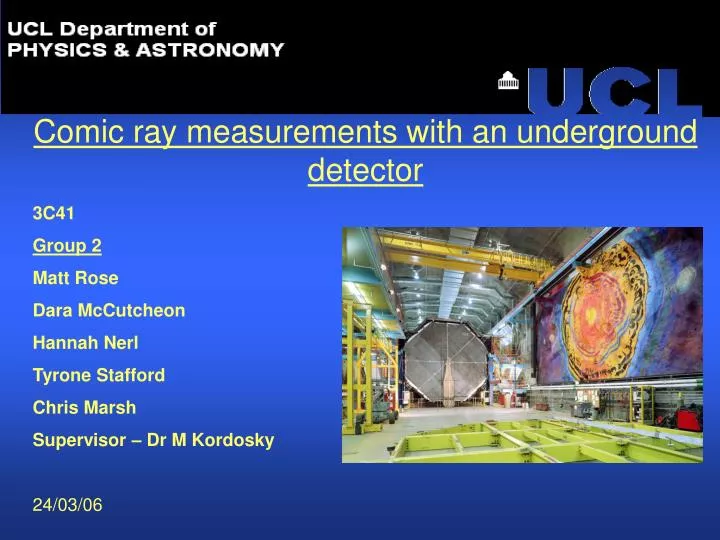
1. Comic ray measurements with an underground detector 3C41 Group 2 Matt Rose Dara McCutcheon Hannah Nerl Tyrone Stafford Chris Marsh Supervisor – Dr M Kordosky 24/03/06

2. Overview of Presentation • Project summary • Introduction to cosmic rays & muons • MINOS detector and science goals • The Moon its orbit and its shadow • Software development • Results • Further ideas Sun shadow – multiple muons

3. The project • Study Cosmic ray secondary muons in the Muon Injector Neutrino Oscillation Search (MINOS) detector. • Look for the Moons shadow in high energy cosmic rays. • Look for the Sun’s shadow. • Study the distribution of multiple muon events.

4. Main obstacles • Accurately plot the Moon’s position relative to MINOS • Getting to the data – familiarisation with Root & C++ • Plot lines in 3D and perform Chi2 tests • Analysis of > 2 million tracks ! • Research into MINOS detector

5. The Moon • As we all know the Moon is made of cheese ! • As it happens cheese is particularly good at stopping cosmic rays! • But seriously the mass of the Moon blocks high energy cosmic rays ( mainly protons ) To observe the shadow of the Moon – - Need to be able to accurately know its position at any one time - Then relate this to events in MINOS • This is not a simple as may first appear, the orbits of the Moon and the Earth are complicated by • Eccentricity in the orbits of the Earth and the Moon • Inclination of the Moon’s orbit • Asymmetry in the gravitational interaction resulting in the Moon rotating synchronously • Internal structure • Librations, • Variable angle subtended for terrestrial observer • Nutation

6. The Moon’s orbit 1 • Eccentricity of the Moon 0.0554 , • Apogee of 406,720 km • Perigee of 356,375 km • Inclination 5.15° to ecliptic • Tides – most well known effect of variable orbit ( +gravitational pertubations from the sun )

7. Moons orbit 2 • Asymmetry in the gravitational interaction resulted in the Moon rotating synchronously (one side facing Earth) • From Earth 59% of the Moon’s surface is visible due to Libration,which has three types Libration in longitude – Caused by the varying orbital velocity relative to Earth axial rotation Libration of latitude – Caused by the Moon’s poles being titled slightly diurnal libration– basically a parallax effect • Nutation Result of eccentricitys in the orbits of the Earth and the Moon and pertubations from the sun. • Angle subtended for terrestrial observer Using the formula h = linear size of object d = distance to observer. Equatorial diameter of the Moon as 3,476 km At Perigee ( 356,375,km), Angular size = 0.536 degrees At Apogee (406,720km),Angular size = 0.470 degrees • Due to these variblitys it was decided to utilise one of the freely avalible programs from the internet and adapt it to our needs

8. Just for interest this is the Far side of the Moon

9. Calculation of the Moon’s Position • Each event in the detector has an associated time • Convert this time into Modified Julian Date (MJD) Julian Date (JD) is the number days elapsed since noon GMT on January 1st 4713 BC plus the decimal fraction of the day since noon MJD = JD – 2400000.5 Now = 53818.48 (MJD)

10. Calculation of the Moon’s Position 2 • Now have Universal Coordinate Time (UTC) in MJD • Convert this to Terrestrial Time (TT) Difference? • - Earth’s rotation is not entirely regular on short time scales • Earth’s rotation is getting longer on large time scales • TT also accounts for relativistic effects TT = UTC + F(UTC)

11. The Moon Zenith North a e East Calculation of the Moon’s Position 3 • Now have TT can calculate the Moon’s position • Was done using a very complicated function that returns topocentric spherical coordinates

12. Calculation of the Moon’s Position 4 • At this point is was both possible and convenient to check that the returned values were accurate • Did so by comparison against the Horizons’ ephemerides (table of astronomical positions in time) Time = Feb,  2, 02:20:10, 2005 Horizons gives:                                a       e  2005-Feb-02 02:20         56.9920 -46.7600  2005-Feb-02 02:21       57.2657 -46.6282 Interpolating for 02:20:10            57.0376 -46.7380 Difference 0.0024   0.0010

13. The Moon Zenith / Z West North Y X Calculation of the Moon’s Position 5 • Rotate coordinate system to match MINOS’s • First convert angles into a unit vector Moon Coordinate System

14. Zenith / Y Θ = 26.6 X Z North Calculation of the Moon’s Position 6 MINOS Coordinate System

15. Zenith Y Zenith / Z Zenith / Z MINOS’s Z North West West West MINOS’s Z MINOS’s Z Y Y X Y X X X Calculation of the Moon’s Position 7 2 1 4 3

16. 1 2 3 4 5 Line fitting of particle tracks u • 486 plates, 8m wide • Each plate 0.024m thick • Alternating layers orthogonal • Strips in each plate 0.04m wide v z • Each strip assigned a ‘number’ • Single layer identifies muon position in a certain strip (u,z) • Adjacent layer pinpoints further its position (v,z) • Interpolation performed by MINOS (u,v,z) for each layer

17. Neutrinos entering the earth have speeds > 0.994c Charge absence and small mass ensure minimal path deviation Results in highly linear tracks Greater error results from resolving power of strips Chi-squared test performed to fit straight line to 3-D data Knowledge of lines equation enables angle of entry of particle to MINOS to be found Linear Fitting Why is it possible to assume only linear tracks are traced?

18. 3-D fitted line & data points x x z 2-D projected line & data points x x x x q x x x x x x x x x x x x x f u v Weighted Least Squares Fitting • Chi-squared is usually applied to 2-D data • Unfortunately no chi-cubed fit appears to exist! • Problem tackled by decomposing 3-D data into 2 sets of 2-D data 2 ‘projected’ lines created: One in u-z plane, one in v-z plane Chi-squared applied to each 2 angles can then be found Information held by 3-D line not lost by working with 2 lines instead

19. Line Fitting Theory • Based on principle of maximum likelihood • This states that:- The ‘best estimate’ or hypothesis for a parameter or parameters is the one which maximises the probability of detecting the outcome that is actually observed in an experiment. • So for n sets of data of the form (ui,zi), a linear correlation is assumed by the standard linear form: zi = mui + c • Values for m, the gradient, and c, the intercept can then be determined

20. Chi - Squared The probability for a particular data set to be observed is given by the complex relation This can only be a maximum when for each set of data points.

21. Chi – Squared 2 • The quantity wi, which is simply the inverse square of the error • is important. This weighting function takes into account the error • on each point. • Points with greater errors contribute less in calculating line properties

22. Calculating Line Properties For those with a mathematical interest • Given • Then and simultaneously • This thus occurs at and • This means and

23. V r b Z α φ a θ U Calculation of the Track Vector

24. Sanity Checks • The orbit of the moon should be periodic, on both a day-to day and lunar cycle scale • The distribution of the angles between a track and the x, y and z axes should be explicable

25. Firstly, the Moon’s Latitude… Over 10 hours, from the sample data Over a larger dataset, approximately three weeks

26. Over a long period… Approximately 28 days, 1 lunar cycle

27. Longitude of the Moon Discontinuous as -180° = 180°

28. For more data, this plot is less helpful… Varies between -180° and 180°

29. Angles between Tracks and MINOS axes • Thx = angle between track and x-axis • Thy = angle between track and y-axis • Thz = angle between track and z-axis

30. Thx • Few tracks parallel to z-axis • Most come from directly above • Cutting out small and poorly fitted tracks sharpens peak

31. Thy • Between 0º and 90º tracks are coming from below • Removing poorly fitted tracks removes small peak • Most tracks coming from between horizon and upward direction

32. Thz • At 0º and 180º, few tracks parallel to z-axis • Less tracks coming from directly above, as they are harder to detect • Removing poorly fitted tracks smoothes edges of the distribution • Assymetric due to the topology of the ground above MINOS!

33. Multiple Muon Events

34. Why look for multiple Muons? • Multiple muon events are not yet fully understood • As a matter of curiosity • To compare with MINOS data • Because we can

35. Three Muon Event A small but significant proportion of MINOS events are multiple muon events

36. Using sample data, occasionally more than one muon was simultaneously observed, but only about 5% of events • It was required to examine a larger data set to try and find higher multiplicity events

37. Multiple muon distribution • Logarithmic scale • The higher multiplicity muon events are less likely • A maximum of 7 simultaneous muons were observed

38. 6 muons • Higher multiplicity events are less frequent • The last Ultra-High Multiplicity event was nearly a year ago MINOS results 23 muons

39. Both the MINOS results and our data suggest that higher multiplicity muon events are less likely • This added functionality may prove useful as more is understood about such events

40. The Sun’s Shadow ?? • A counter intuitive statement ?! Looking for deficiency in Galactic cosmic rays compared to solar cosmic rays. • Similar angular scale compared with the moon -> eclipses • GCR have a power law distribution γ =2 .7 for energies < 10^6 GeV & γ = 3 > 10^6 • SCR lower energy than GCR. SCR produced in solar flares (1- 10 KeV) and Coranol mass ejections (upto 300 KeV) – spectrum less well understood ( although significantly less energy than GCR )

41. Sun shadow 2 • To observe the solar shadow may require analysis of energy and angular distribution to differentiate between types Magnetic effects • Geomagnetic and Heliomagnetic fields will distort the paths of incoming cosmicrays. Dependant on both speed of particles and strength of magnetic fields Weather dependent! ie different for solar maximum/minimum The Forbush decrease • At solar maximum the SCR have their highest flux, the increase in SCR is accompanied by a decrease in the GCR. This relationship between the two types of cosmic rays is called the Forbush decrease. The Forbush decrease is caused by the magnetic field of the solar wind plasma sweeping GCR away from Earth.

42. Thank you for listening