Download
1 / 37
510 likes | 1.54k Vues
Stress, Strain, Pressure, Deformation, Strength, etc. Maurice Dusseault. Stresses (I). Stresses in a solid sediment arise because of gravity and geological history Stresses are different in diffferent directions

E N D
Stress, Strain, Pressure, Deformation, Strength, etc. Maurice Dusseault
Stresses (I) • Stresses in a solid sediment arise because of gravity and geological history • Stresses are different in diffferent directions • Three principal stresses are orthogonal, and the vertical direction is usually one of them • Overburden weight is = v (+/- 5%) • The lateral stresses, hmin and HMAX (or h and H) are at 90 degrees to one another
Stresses (II) • Normal stresses () act orthogonal to a plane and cause the material to compress • Shear stresses () act parallel to a plane and cause the material to distort y- yx Static equilibrium: xx yy xy = - yx xy x+ x - xy yx y+
Pressures • Pressures refer to the fluid potential (p) • Pressures can be hydrostatic, less than hydrostatic (rare) or greater (common). Called underpressured or overpresssured • Pressures at a point are the same in all directions because they are within the fluid • We assume that capillary effects are not important for large stresses and pressures • Differences in pressures lead to flow
Pressures at Depth pressure (MPa) Fresh water: ~10 MPa/km Sat. NaCl brine: ~12 MPa/km ~10 MPa Hydrostatic pressure distribution: p(z) = rwgz 1 km Underpressured case: underpressure ratio = p/(rwgz), a value less than 1 Overpressured case: overpressure ratio = p/(rwgz), a value greater than 1.2 underpressure overpressure Normally pressured range: 0.95 < p(norm) < 1.2 depth
Effective Stress () Principle • The famous Terzaghi concept (1921) • Only “effective” stresses [’ ] affect strength and deformation behaviour • Effective stress is the stress component transmitted through the solid rock matrix • Total stresses are the sum of the effective stresses and the pressures: = + p, or: ij = []ij + [p]
sv + po = sv (or Sv) f1 f4 sh + po = sh (or Sh) sh + po = sh (or Sh) f2 po f3 sv + po = sv (or Sv) Effective Stresses • Pressure is the same in all directions (a fluid) • Effective stress is the sum of the grain-to-grain (matrix) forces • The sum of p and s gives total stresses, s • Usually, sv = r(z)dz • shmin , sHMAX must be measured or estimated
Rock Strength (I) • Strength is the resistance to shear stress (shear strength), compressive normal stress (crushing strength), tensile stress (tensile strength), or bending stress (beam strength). • All of these depend on effective stresses (), therefore we must know the pore pressure (p) • Rock specimen strength is usually very different than rock mass strength because of joints, bedding planes, fissures, etc. • Which to use? Depends on the problem scale.
F F Rock Strength (II) • Tensile strength (To) is extremely difficult to measure: it is direction-dependent, flaw-dependent, sample size-dependent, ... • To is used in fracture models (HF, thermal fracture, tripping or surge fractures) • For a large reservoir, To may be assumed to be zero because of joints, bedding planes, etc. Prepared rock specimen A To = F/A
Rock Strength (III) • Shear strength is a vital geomechanics strength aspect, often critical for design • Shearing is associated with: • Borehole instabilities, including breakouts, failure • Reservoir shear and induced seismicity • Casing shear and well collapse • Reactiviation of old faults, creation of new ones • Hydraulic fracture in soft, weak reservoirs • Loss of cohesion and sand production • Bit penetration, particularly PCD bits n slip plane sn is normal effective stress t is the shear stress plane rock
Rock Strength (IV) a slip planes • Shear strength depends on the frictional behaviour and the cohesion of the rock • Carry out a series of triaxial shearing tests at different 3, plot each as a stress-strain curve, determine peak strengths r r a 1 - 3 peak strength stress difference a axial strain
1 - 3 Curves peak strength massive damage, shear plane develops damage starts sudden stress drop (brittle) cohesion breaking stress difference continued damage ultimate or residual strength “elastic” part of curve a seating, microcrack closure axial strain
Rock Strength (V) • To plot a yield criterion from triaxial tests, plot 1, 3 at failure on equally scaled n axes, join with a semicircle, then sketch tangent (= Y) • Y cohesion c n To 3 1
1 Curved or linear fit tan2 Uniaxial compressive strength, C0 3 13Plotting Method • Plot 1, 3 values at peak strength on axes • Fit a curve or a straight line to the data points • The y-intercept is the unconfined strength Y = (1 - 3tan2 - C0 = 0) (straight line approximation)
Rock Strength (VI) • Strength of joints or faults require shear box tests • Specimen must be available and aligned properly in a shear box • Different stress values (N) are used Area - A N - normal force S Shear box S - shear force N S A Linear “fit” Curvilinear “fit” data point N c A cohesion
S = t A Linear “fit” Curvilinear “fit” data point N c A cohesion = sn Yield Criterion • This type of plot is called a Mohr-Coulomb plot. Y is usually called a Mohr-Coulomb “yield” or “failure” criterion • It represents the shear strength of the rock (S/A) at various normal stresses (N/A), A is area of plane • For simplicity, a straight line fit is often used Y
Cohesion • Bonded grains • Crystal strength • Interlocking grains • Cohesive strength builds up rapidly with strain • But! Permanently lost with fabric damage and debonding of grains 1 - 3 complete s-e curve cohesion mobilization stress difference friction mobilization a
Friction • Frictional resistance to slip between surfaces • Must have movement () to mobilize it • Slip of microfissures can contribute • Slip of grains at their contacts develops • Friction is not destroyed by strain and damage • Friction is affected by normal effective stress • Friction builds up more slowly with strain mob = cohesion + friction f = c + n
Estimating Rock Strength • Laboratory tests OK in some cases (salt, clay), and are useful as indicators in all cases • Problems of fissures and discontinuities • Problems of anisotropy (eg: fissility planes) • Often, a reasonable guess, tempered with data, is adequate, but not always • Size of the structure (eg: well or reservoir) is a factor, particularly in jointed strata • Strength is a vital factor, but often it is difficult to choose the “right” strength value
0° 30° 60° 90° Strength Anisotropy UCS UCS Vertical core Bedding inclination
Crushing Strength (I) • Some materials (North Sea Chalk, coal, diatomite, high porosity UCSS) can crush • Crushing is collapse of pores, crushing of grains, under isotropic stress (minimal ) • Tests involve increasing all-around effective stress (’) equally, measuring V/’ • Tests can involve reducing p in a highly stresses specimen (ie: ’ increases as p drops) UCSS = unconsolidated sandstone
Crushing Strength (II) • Apply p, ( > p), allow to equilibrate ( = - p) • Increase by increasing or dropping p = - p • Record volumetric strain, plot versus effective stress • The curve is the crushing behavior with + V p LE crushing material V
Rock Stiffness • To solve any ’-problem, we have to know how the rock deforms in response to a stress change • This is often referred to as the “stiffness” • For linear elastic rock, only two parameters are needed: Young’s modulus, E, and Poisson’s ratio, (see example) • For more complicated cases, more parameters are required
Rock Stiffness Determination • Stiffness controls stress changes • Estimate stiffness using correlations based on geology, density, porosity, lithology, .... • Use seismic velocities (vP, vS) for an upper-bound limit (invariably an overestimate) • Use measurements on laboratory specimens (But, there are problems of scale and joints) • In situ measurements (THE tool, others ...) • Back-analysis using monitoring data
L strain () = L E = What are E and ? deformation L Young’s modulus (E): E is how much the material compresses under a change in effective stress radial dilation r L Poisson’s ratio is how much rock expands laterally when compressed. If = 0, no expansion (eg: sponge) In = 0.5, complete expansion, therefore volume change is zero r = L
Rock Properties from Correlations • A sufficient data base must exist • The GMU must be properly matched to the data base; for example, using these criteria: • Similar lithology • Similar depth of burial and geological age • Similar granulometry and porosity • Estimate of anisotropy (eg: shales and laminates) • Correlation based on geophysical properties (KBES) • Use of a matched analogue advised in cases where core cannot be obtained economically GMU = geomechanical unit
What is a Matched Analogue? • Rocks too difficult to sample without damage, or too expensive to obtain • Study logs, mineralogy, even estimate the basic properties (f, E, n…) • Find an analogue that is closely matched, but easy to sample for laboratory specimens • Use the analogue material as the basis of the test program • Don’t push the analogue too far!!
Seismic Wave Stiffness • vP, vS are dynamic responses affected by rock density and elastic properties • Because seismic strains are tiny, they do not compress microcracks, pores, or contacts • Thus, ED and D are always higher than the static test moduli, ES and S • The more microfissures, pores, point contacts, the more ED > ES,x 1.3, even to x 10 • If porosity ~ 0, very high, ES approaches ED
Laboratory Stiffness • Cores and samples are microfissured; these open when stress is relieved, E may be underestimated • In microfissured or porous rock, crack closure, slip, and contact deformation dominate stiffness • ES and S under confining stress are best values • Joints are a problem: if joints are important in situ, their stiffness may dominate rock response, but it is difficult to test in the laboratory
Cracks and Grain Contacts (I) E2 E1 Microflaws can close, open, or slip as changes E1 E3 • Flaws govern rock stiffness The nature of the grain-to-grain contacts and the overall porosity govern the stiffness of porous SS
Cracks and Grain Contacts (II) • Point-to-point contacts are much more compliant than long (diagenetic) contacts • Large open microfissures are compliant • Oriented contacts or microfissures give rise to anisotropy of mechanical properties • Rocks with depositional structure or exposed to differential stress fields over geological time develop anisotropy through diagenesis
How Do We “Test” This Rock Mass? • Joints and fractures can be at scales of mm to several meters • Large core: 115 mm • Core plugs: 20-35 mm • If joints dominate, small-scale core tests are “indicators” only • This issue of “scale” enters into all Petroleum Geomechanics analyses A large core specimen A core “plug” 1 m Machu Picchu, Peru, Inca Stonecraft
Induced Anisotropy • UCSS# subjected to large stress differences develops anisotropy (contacts form in 1 direction and break in 3 direction) • A brittle isotropic rock develops microcracks mainly parallel to 1 direction • Now, these rocks have developed anisotropy because of their -history (i.e.: damage) • This is a challenging area of analysis # UCSS = unconsolidated sandstone
In Situ Stiffness Measurements • Pressurization of a packer-isolated zone, with measurement of radial deformation • Direct borehole jack methods (mining) • Geotechnical pressuremeter modified for high pressures (membrane inflated at high pressure, radial deformation measured) • Correlation methods (penetration, indentation, others?) • These are not widely used in Petroleum Eng.
Back-Analysis for Stiffness • Apply a known effective stress change, measure deformations (eg: uplift, compaction) • Use an analysis model to back-calculate the rock properties (best-fit approach) • Includes all large-scale effects • Can be confounded by heterogeneity, anisotropy, poor choice of GMU, ... • Often used as a check of assumptions
Direct Borehole Stability Problems • Stuck drill pipe • differential pressure sticking • wedging in the borehole • Stuck casing during installation • Lost circulation (in many cases) • Mudrings, cuttings build-up in washouts • Borehole squeeze
Indirect Stability Problems • Slow advance rates in drilling • Longer hole exposure = greater costs • Longer exposure = greater chance of instability • Solids build-up and loss of mud control • Blowouts • Washouts, sloughing cause tripping and drilling difficulties, swabbing • A blowout eventually develops as control is lost