Download

1 / 27
270 likes | 288 Vues
Learn advanced memory optimization aspects of A* search algorithms, including Iterated Deepening A*, Iterative-Deepening A*, Simplified Memory-Bounded A*, f1, f2, f3, and f4 extensions. Understand how to set f-bounds, perform f-limited search, and utilize Iterative Deepening A*. Explore properties and examples of IDA* and Simplified Memory-Bounded A*. Discover the trade-offs between memory usage and optimality in search algorithms.

E N D
More advanced aspects of search Extensions of A* Concluding comments
Extensions of A* Iterated deepening A* Simplified Memory-bounded A*
f1 A* d = 1 Breadth- first f2 d = 2 d = 3 f3 d = 4 f4 Expand by depth-layers Expands by f-contours Memory problems with A* • A* is similar to breadth-first: • Here: 2 extensions of A* that improve memory usage.
Depth-first in each f- contour • Perform DEPTH-FIRST search LIMITED to some f-bound. • If goal found: ok. • Else: increase de f-bound and restart. f1 f2 f3 f4 Iterative deepening A* How to establish the f-bounds? - initially: f(S) generate all successors record the minimalf(succ)>f(S) Continue with minimalf(succ) instead of f(S)
f-new = 120 S f=100 A f=120 B f=130 C f=120 D f=140 G f=125 E f=140 F f=125 Example: f-limited, f-bound = 100
f-new = 125 S f=100 A f=120 B f=130 C f=120 D f=140 G f=125 E f=140 F f=125 Example: f-limited, f-bound = 120
S f=100 A f=120 B f=130 C f=120 D f=140 G f=125 E f=140 F f=125 SUCCESS Example: f-limited, f-bound = 125
f-limited search: 1. QUEUE <-- path only containing the root; f-bound <-- <some natural number>; f-new <-- 2. WHILEQUEUE is not empty AND goal is not reached DO remove the first path from the QUEUE; create new paths (to all children); reject the new paths with loops; add the new paths with f(path)f-bound to front of QUEUE; f-new <-- minimum of current f-new and of the minimum of new f-values which are larger than f-bound 3. IF goal reached THEN success; ELSE report f-new ;
1. f-bound <-- f(S) 2. WHILE goal is not reached DO perform f-limited search; f-bound <-- f-new Iterative deepening A*:
Properties of IDA* • Complete and optimal: • under the same conditions as for A* • Memory: • Let be the minimal cost of an arc: • == O( b* (cost(B) /)) • Speed: • depends very strongly on the number of f-contours there are !! • In the worst case: f(p) f(q) for every 2 paths: • 1 + 2 + ….+ N = O(N2)
In absence of Monotonicity: • we can have search spaces like: 100 S 120 120 A B C D E F 140 150 90 60 • If f can decrease, • decreasing nodes can not be goal nodes: they are “rubbish” nodes, taken away in the same iteration. Why is this optimal,even without monotonicity ??
IDA* is one of the very best optimal search techniques ! • Example: the 8-puzzle • But: also for MANY other practical problems • increase f-bound by a fixed number at each iteration: • effects: less re-computations, BUT: optimality is lost: obtained solution can deviate up to Properties: practical • Ifthere are only a reduced number of different contours: • Else, the gain of the extended f-contour is not sufficient to compensate recalculating the previous • In such cases:
If memory is full and we need to generate an extra node (C): • Remove thehighest f-value leaffrom QUEUE(A). • Remember thef-value of the best ‘forgotten’ childin each parent node(15 in S). 13 S 13 15 A B B 18 C memory of 3 nodes only Simplified Memory-bounded A* • Fairly complex algorithm. • Optimizes A* to work within reduced memory. • Key idea: (15)
When expanding a node (S), only add its children 1 at a time to QUEUE. • we use left-to-right • Avoids memory overflow and allows monitoring of whether we need to delete another node 13 S A A B B First add A, later B Generate children 1 by 1
If extending a node would produce a path longer than memory: give up on this path (C). • Set the f-value of the node (C) to • (to remember that we can’t find a path here) 13 S 13 B B 18 C C D memory of 3 nodes only Too long path: give up
If all children M of a node N have been explored and for all M: • f(S...M)f(S...N) • then reset: • f(S…N)= min { f(S…M) | M child of N} • A path through N needs to go through 1 of its children ! 15 13 S 24 15 A B Adjust f-values better estimate for f(S)
0+12=12 10 S 8 8+5=13 10+5=15 A B 8 16 10 10 20+0=20 16+2=18 20+5=25 24+0=24 C G1 D G2 8 10 10 8 30+5=35 24+5=29 E G3 30+0=30 G4 F 24+0=24 12 12 12 13 S S S S A A A B A B 13 13 15 15 15 15 D 18 SMA*: an example: 12 13 (15)
0+12=12 10 S 8 8+5=13 B 10+5=15 A B 13 8 16 10 10 20+0=20 16+2=18 20+5=25 24+0=24 C G1 D G2 8 10 10 8 D 24+0=24 30+5=35 24+5=29 E G3 30+0=30 G4 F (15) 13 (15) 15 15 15 (24) 13 (15) S S S S S 13 B B B B A A A () 15 24 24 24 15 15 G2 G2 G2 C C C G1 D D 24 24 24 25 20 Example: continued 15 (15) (24) 20 13 15 () 13 20 () () 24 15
SMA*: properties: • Complete: If available memory allows to store the shortest path. • Optimal: If available memory allows to store the best path. • Otherwise: returns the best path that fits in memory. • Memory: Uses whatever memory available. • Speed: If enough memory to store entire tree: same as A*
Concluding comments More on non-optimal methods The optimality Trade-off
8 4 7 8 1 better than 5 5 3 4 3 6 1 7 2 6 2 Non-optimal variants • Sometimes ‘non-admissible’ heuristics desirable: • Example: symmetry • but cannot be captured with underestimating h • = Use non-admissible A*.
f(S…N) = * cost(S…N) + h(N) ,0 1 = 0 : pure heuristic best first (Greedy search) = 1 : A* Non-optimal variants (2) • Reduce the weight of the cost in f:
Polynomial parallel algorithms exist, but ALL KNOWN sequential algorithms are exponential • The trade-off: • either use algorithms that; • ALWAYS give the optimal path Approaching the complexity • Optimal path finding is by nature NP complete ! • in the worst case (depending on the actual search space !) , behave exponential • in the average case are polynomial
Complexity continued: • OR, use algorithms that: • ALWAYS produce solutions in polynomial time • in the worst case (actual search space), the solution is far form the optimal one • in the average case, it is close to the optimal one • Examples: local search, non-admissible A*, 1 .
city1 N-1 city2 city3 ... cityN-1 ... N-2 ... ... • Speed: ~ N 2(= 1 + 2 + 3 …+ N-1) Example: traveling salesmanwith minimal cost • Assume there are N cities: • Worst case: • solution found/ best solution log2(N+1)/2 • Average case: • solution found ~ 20% longer than best