Macroeconomic Theory

Macroeconomic Theory Chapter 1 Motivation for Macroeconomic models?

Macroeconomic models help us in framing key questions that face macroeconomists: • How are the levels of output and employment are determined and why they fluctuate? • Why does inflation occur and when should we worry about it? • How does government policy affect inflation and unemployment? • Why unemployment is high for lengthy periods in some countries than others? • How do trade, international financial markets and exchange rates affect employment and inflation? • Why are some countries are rich and others are poor?

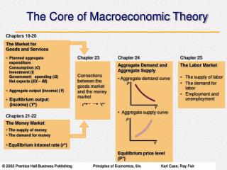
Output, unemployment and inflation The 3 equation model • IS curve “aggregate demand” • PC curve “supply side of the economy” • MR “the behavior of inflation targeting central bank What do we mean by impact on the economy? • We mean impact on output, unemployment and inflation. The basic model must answer the following questions: • how actual output and employment is determined • What determines employment at which inflation is stable (medium run eq. level of employment • How the economy adjusts from current position to medium run eq. and what factors influence the speed and smoothens of adjustment.

Assumptions and terminology • A special feature of macroeconomics is that the behavior of different agents has to be taken into account simultaneously: • Actions of households (to enter the labor force, to spend, to save ..etc) • Actions of firms (set wages, invest .. etc) • Actions will be sensitive to government actions (T, G, interest policy), current economic variables and expectations of these variables such as tax, wages…etc.

Aggregate supply side: refers to the supply of goods and services. The supply side consists of: • Factors of production • Technology • The way which incomes (workers and firms) are determined • Aggregate demand side Refers to aggregate demand for goods and services and consists of: • C, I, and G

C is the expenditure of individuals on goods and services (durable or non-durables) • I expenditures of capital goods mostly by firms. New housing and spending by the government on machinery are also I. • G on salaries, purchase of goods and services. • Short run (months) • A period during which aggregate demand, output and employment can change but before prices and wages respond to the change in output and employment (assuming they are given), i.e., they are fixed or sticky or rigid. • Assuming that wages and prices are given can also refer to the case when they change by a constant amount.

Therefore in the short run, wages and prices or their rate of change do not respond to changes in the level of output, it also means that it is aggregate demand that determines the level of output and employment. • Medium run • The period during which wages and prices can respond to changes in output and employment. The supply side of the economy adjusts to establish a medium run equilibrium in which inflation is constant. • Capital stock (and technology) and the labor force (population and migration, i.e., the supply side of the labor market) are also constant.

The attention is focused on the behavior of wages and price setters. No upward or downward pressure on wages or prices. • Long run: investigates the consequences of changes in technology such as productivity growth. The growth theory. Here we allow for population, physical capital and technology to change. • Market imperfections (market power, lack of complete information.

Fluctuations in output and employment • See fig. 1.1. (compare between US and France) swings from peak to trough is called business cycle. • In the short run, the level of output depends on aggregate demand. • Fig. 1.2 shows unemployment in US and Europe • The IS/LM model will help us to understand the factors that influence AD.

Figure 1.1

Figure 1.2

Unemployment: International Comparisons • Fig. 1.3 shows trends of unemployment in 7 countries. • There is a rising rate in Europe between 1970s-1990s. • There is a striking difference between US and European economies • The idea of a roughly constant equilibrium unemployment rate is plausible for US (6%) and Japan. • Till 1980s the European unemployment was lower than US. • There is a significant variability in unemp. rates. • Swedish unemployment rate is different. • Japan’s rate was very low till early 1990s.

Figure 1.3

Modeling medium run unemployment • In the competitive model, labor market clears, i.e. real wage adjusts so that the demand for labor equals its supply, and firms are in equilibrium. • On the demand side, it is not profitable to employ more or less labor. • On the supply side there will be no more supply of labor or less supply. • The only kind of unemp in the competitive market is voluntary unemp workers choose not to work because they derive more utility from being unemployed, i.e., they preferleisure. • The rate of unemp that corresponds to the market clearing level is the competitive equilibrium rate of unemp.

Imperfect Competition Model • In an imperfect competition model the equilibrium labor market does not necessarily coincide with market clearance. There can be involuntary unemployment even at equilibrium. • In an imperfect competition model we can talk of wage setters (employees or unions) and price setters (firms). • Firms can earn supernormal profit. The price set by the firm is above MC and the difference is the profit the firm makes. • With imperfect competition money wages will be set by employers or unions or by both • The real wage will depend both on the outcome of wage setting and the price setting across the country, and will be higher than perfect competition level. One explanation is the collective bargaining power of employees will result in a wage that is higher than the minimum an employee would work for. • The imperfectly competitive eq unemp rate is the level at which both wage and price setters accept the prevailing real wage.

Inflation • In an economy with constant inflation, it will be in a medium run equilibrium, eq rate of unemployment “ERU”. • If AD rises output and employment will rise, unemp will be below ERU. • Workers will be in a stronger bargaining position and real wages have to rise. Current real wage is lower than what wage setters will be satisfied with. Wage setters raise money wages • Price setters will not be satisfied as this will raise their costs. To maintain their profits they will have to raise their prices. • AD that raises output and employment above eq leads to a rise in inflation. • Can lower unemp and higher inflation be sustained by the government setting its policy to achieve this. This will depend on whether the labor market is competitive. In a competitive labor market if employment is higher than the level at which labor supply and demand are equal, the wage rate will either be too low from the labor supply side or too high for firms.

When unemp is below ERU and inflation is up. Wage and price setters are not in eq, wage setters would raise wages as their living standards reduced. Raising money wages will raise inflation even further. • Look at fig. 1.4. In USA inflation is smooth in the post 1950s.

Figure 1.4

Inflation and Monetary Policy • Monetary policy in some countries was directed at reducing unemp, in other countries to an inflation target. • Suppose that the CB policy is to set interest rates so as to steer the economy to a low target rate of inflation. In response to inflation it would put up interest rate, which ↓ AD as I ↓ due to higher interest rate, this in turn ↓ emp and inflationary pressures. • Fig 1.5 provides a schematic overview of the short and medium run macro model.

Figure 1.5

Economic Growth

Growth and diminishing returns to factor accumulation • What determines the outputper worker. In the short and medium run it is assumed that the amount of capital available to worker is fixed. In the long run the level of output per worker depends on capital available. Human capital should also be included (through education, training ..etc.). Technology and efficiency matter as well. • The neoclassical theory of economic growth was developed by Solow and Swan, it focused on systematizing the role of factor accumulation in growth. The essence of the Solow/Swan model is that the level of output per head would be higher if there was a higher level of capital per worker. • The model predicts that more investment would only raise the growth rate of living standards temporarily, because it assumes that there are diminishing returns to physical investment.

With more investments capital intensive techniques will be adopted, output per worker ↑ but with each increase in capital intensity, the bonus in terms of higher output per worker diminishes, because part of the capital stock disappears through depreciation and feeble improvements in output will not generate sufficient extra savings to raise capital intensity. • Note the following: • The model can be amended by including a particular kind of technical progress: if technology is improving year on year without using up any resources, we can say that there is exogenous technical progress. In this case output per head rises at this constant exogenous rate.

When investment ↑ there is a period during which output per head rises faster than the rate of exogenous technical progress because of increases in capital intensity. Eventually the economy will return to the original rate of growth, with a higher living standards than what would have been the case in the absence of the shift in higher investment. • The model helps explain why should be a positive relationship between output per head and capital per head. But it does not predict correctly by how much a rise in capital per head will raise output per head. • This question focuses attention on • The need to include human as physical capital as a factor of production in the growth model. • Whether all countries have access to the same technology • Whether even if they do, the technology can be used efficiently

Growth and constant returns to factor accumulation • Dissatisfaction with the role of exogenous technical progress in the Solow/Swan model motivated the endogenous growth theory. • Drop the assumption of diminishing returns to the accumulation of capital and replace it with an assumption of constant returns. • If the economy devotes higher investment this raises the growth rate of the output per head permanently. This transforms the process of growth into endogenous growth. • Why returns to factor accumulation may not diminish? One idea focuses on human capital, spending more time in education can raise the growth rate permanently, as well as higher investment in innovative activities.

Innovation and incentives: Schumpeterian growth • Schumpeter argued that innovations could sustain long-run growth and that institutions are important for creating the appropriate incentives for firms to engage in innovative activities. • Ideas are a different form fixedcapital: once an idea has been developed, use of it by one does not prevent others from using it too, as ideas are “not rival”. In the Schumpeterian model, countries can be trapped with low levels of GDP per capita because the institutional structures are not conductive to taking advantage of spillovers in innovation from rich countries.

Macroeconomic Theory