Ray Tracing
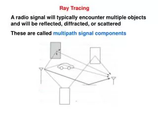
Ray Tracing. A radio signal will typically encounter multiple objects and will be reflected, diffracted, or scattered These are called multipath signal components. Represent wavefronts as simple particle Geometry determines received signal from each signal component

Ray Tracing
E N D
Presentation Transcript
Ray Tracing A radio signal will typically encounter multiple objects and will be reflected, diffracted, or scattered These are called multipath signal components
Represent wavefronts as simple particle • Geometry determines received signal from each signal component • Typically includes reflected rays, can also include scattered and diffracted rays • Requires site parameters • Geometry • Dielectric properties • Error is smallest when the receiver is many wavelengths from the nearest scatterer and when all the scatterers are large relative to a wavelength
Accurate model under these conditions • Rural areas • City streets when the TX and RX are close to the ground • Indoor environments with adjusted diffraction coefficients • If the TX, RX, and reflectors are all immobile, characteristics are fixed • Otherwise, statistical models must be used
Two – Ray Model Used when a single ground reflection dominates the multipath effects. • Approach: • Use the free – space propagation model on each ray • Apply superposition to find the result
time delay of the ground reflection relative to the LOS ray product of the transmit and receive antenna field radiation patterns in the LOS direction
product of the transmit and receive antenna field radiation patterns corresponding to x and x’, respectively R = Ground reflection coefficient
Delay spread = delay between the LOS ray and the reflected ray
If the transmitted signal is narrowband wrt the delay spread
d = Antenna separation h t = Transmitter height h r = Receiver height
When d is large compared to h t + h r : Expand into a Taylor series
The ground reflection coefficient is given by vertical polarization horizontal polarization for ground, pavement, etc...
As d increases, the received power • Varies inversely with d 4 • Independent of
f = 900 MHz R = - 1 h t = 50 m h r = 2 m Gl = 1 G r = 1 P t = 0 dBm
The path can be divided into three segments • d < h t • The two rays add constructively • Path loss is slowly increasing • Path loss
h t < d c • Wave experiences constructive and destructive interference • Small – scale (Multipath) fading • If power is averaged in this area, the result is a piecewise linear approximation • d c < d • Signal power falls off by d – 4 • Signal components only combine destructively
To find d c , set • In segment 1, d < h t power falls off by • In segment 2, h t < d < d c power falls off by – 20 db/decade • In segment 3, d c < d, power falls off by – 40 db/decade • Cell sizes are typically much less than d c and power falls off by
Problem 2 – 5 Find the critical distance, d c , under the two – ray model for a large macrocell in a suburban area with the base station mounted on a tower or building (h t = 20 m), the receivers at height h r = 3 m, and f c = 2 GHz. Is this a good size for cell radius in a suburban macrocell? Why or why not? Solution
Ten – Ray Model (Dielectric Canyon) • Assumptions: • Rectilinear streets • Buildings along both sides of the street • Transmitter and receiver heights close to street level • 10 rays incorporate all paths with 1, 2, or 3 reflections • LOS (line of sight) • GR (ground reflected) • SW (single wall reflected) • DW (double wall reflected • TW (triple wall reflected) • WG (wall – ground reflected) • GW (ground – wall reflected)
Overhead view of 10 – ray model x i = path length of the i th reflected ray Product of the transmit and receive antenna gains of the i th ray
Assume a narrowband model such that for all i • Power falloff is proportional to d - 2 • Multipath rays dominate over the ground reflected rays that decay proportional to d - 4
General Ray Tracing • Models all signal components • Reflections • Scattering • Diffraction • Requires detailed geometry and dielectric • properties of site • Site specific • Similar to Maxwell, but easier math • Computer packages often used • The GRT method uses geometrical optics to trace the propagation of the LOS and reflected signal components
Shadowing: Diffraction and Spreading Diffraction • Diffraction occurs when the transmitted signal "bends around" an object in its path • Most common model uses a wedge which is asymptotically thin • Fresnel knife – edge diffraction model
For h small wrt d and d', the signal must travel an additional distance d The phase shift is
is called the Fresnel – Kirchhoff diffraction parameter Approximations for the path loss relative to LOS are
Okumura model • Empirically based (site/freq specific) • Awkward (uses graphs) • Hata model • Analytical approximation to Okumura model • Cost 136 Model: • Extends Hata model to higher frequency (2 GHz) • Walfish/Bertoni: • Cost 136 extension to include diffraction from rooftops
Simplified Path – Loss Model K = dimensionless constant that depends on the antenna characteristics and the average channel attenuation d 0 = reference distance for the antenna far field = path – loss exponent LOS, 2 – ray model, Hata model, and the COST extension all have this basic form
Generally valid where d > d 0 d 0 = 1 – 10 m indoors = 10 – 100 m outdoors • General approach: • Take data at three values of d • Solve for K, d o , and