Wireless Localization using Self-Organizing Maps
Solve localization problem in wireless sensor networks with algorithms. Discover services, ensure security, and navigate accurately. Explore range-free and range-based techniques for precise results. Resolve ambiguities in embedding with known edge lengths. Study spring-mass model for network accuracy.


Wireless Localization using Self-Organizing Maps
E N D
Presentation Transcript
Wireless Localization using Self-Organizing Maps S. K. S. Gupta School of Computing and Informatics Arizona State University Tempe, AZ Joint work with G. Giorgetti and G. Manes – U. of Frienza
Location awareness: • Enable Context-Aware Apps • Resource & Services Discovery • Tracking (People, Equipment,...) • Navigation Support • Security (Location-based access) 4 6 9 7 2 10 3 8 0 1 5 Localization Problem: to assign coordinates to the network nodes Fire! Quick solutions: • Manual Configuration: not feasible for large networks. • GPS: accurate, but power-hungry and not cost-effective Need of Localization Algorithms for Wireless Sensor Networks Remote user
Single-Hop Localization In the simplest case, localization consists in computing the position of a single node based on measurements from nodes at fixed positions. Range-Free: Range-Based: Scene Analysis: Proximity Angulation, Multilateration, Triangulation WiFi and GPS fingerprinting
Multi-hop Localization • In general, solving the localization problem requires to compute the positions of a set of nodes. • Scene analysis is not applicable if the coverage of anchor nodes is partial. • Range-free and range-based techniques are still applicable, but the problem become more complex (see next…) • Anchor-Free localization can be used to derive relative positions of node in absence of reference points (still useful, see next…).
Virtual Coordinates If no anchor information is used, the map produced by the localization algorithm will be arbitrarily rotated, translated or flipped. Node positions are expressed in terms of Virtual Coordinates. Note that although the true positions are not known, nodes with similar virtual coordinates are close in space. GeoRouting: at each step, forward the packet to the node with virtual coordinates closer to the destination point. Service Discovery: locate the service (e.g. a printer) closer to the user.
The problem: locating the nodes Inputs: • A set of nodes: 6 4 8 1 3 10 9 5 2 7 0 2) A set of measurements: e.g. Range measurements: d(p1,p2) = Z12 e.g. Connectivity constraints d(p3,p4) ≤ Z34 Output: a set of node coordinates
2 7 1 4 5 3 8 6 Graph Embedding in Euclidean Spaces WSN represented as a undirected graph G=(V,E) GRAPH EMBEDDING: find a mapping :V Rd such that the the computed coordinates satisfy constraints (e.g. graph planar, or edge have specific lengths ) The problem has been extensively studied due to its application to molecular conformation, structural analysis, graph drawing.
d(3,4) 5 3 d(3,6) 8 d(5,6) d(3,8) 6 2 2 2 d(1,2) d(1,2) d(1,2) d(2,4) d(2,4) d(2,4) 7 7 7 4 1 1 1 4 4 d(4,5) d(4,5) d(4,5) d(3,4) d(3,4) d(3,4) d(5,7) d(5,7) d(5,7) 5 5 5 d(1,3) d(1,3) d(1,3) 3 3 3 d(3,6) d(3,6) d(3,6) 8 8 8 d(5,6) d(5,6) d(5,6) d(3,8) d(3,8) d(3,8) 6 6 6 Uniqueness of the Solution d(1,3) Original graph Translation Rotation Reflection If we use inter-node distances, the solution is correct up to global translation, rotation or reflection. We need to fix the relative position of 3 non collinear nodes (2D). These ambiguities arise with anchor-free localization (only the relative positions are computed).
2 d(1,2) d(2,4) 7 d(4,5) 1 4 d(3,4) d(5,7) 5 d(1,3) 3 d(3,6) 8 d(5,6) d(3,8) 6 Embedding with known edge lengths We assume that inter-node distances can be measured. Note: this is feasible only if nodes have dedicated hardware (e.g. ultrasound). • Problem: • find an embedding such that d(p1,p2)=d((1), (2)) • Fundamental Questions: • Computational complexity • Uniqueness of solution • Answer 1: • Graph Embedding is NP-complete in 1D and NP-hard in 2D [Saxe79]
6 7 7 Uniqueness of the Solution (cntd) Considering N nodes there are 2N degree of freedom in the 2D space. Each measurement set a constraint. If we don’t have enough constraints the solution is not unique. 2 7 1 4 2 5 7 3 1 4 8 5 3 8 6 Flexible framework 6 Flipping ambiguities
2 d(1,2) d(2,4) 7 d(4,5) 1 4 d(3,4) d(5,7) 5 d(1,3) 3 d(3,6) 8 d(5,6) d(3,8) 6 Condition for unique realization in 2D • The graph need to have 2N-3 well distributed edges [2] • The graph need to be triconnected and reduntantly ridig [3] • Condition are testable in polynomial time (peeble game) [5] • This conditions were proved to be necessary and sufficient [4] • No such characterization exists for dimension greater than 2
Connectivity information only R • Assuming an idealized radio model: • d(a,b) ≤ R a,b neighbors • d(a,c) > R a,c non neighbors • Network can be represented by an Unit Disk Graph (UDG) 2 7 1 4 5 3 8 6 NB(3)={1,2,4,6,8) • Theoretical Results on Unit Disk Graphs: • Embedding NP-Complete in 1D and NP-hard in 2D [6] • Problem is APX-hard (no Polynomial Time Approximation) [7] • Finding exact nodes position is not just hard algorithmically, but impossible since the lack of information
Spring-Mass Model The network is modelled as a mesh of masses connected by spring with a given length. The springs push or pull the nodes until the internode distance are correct. Localization code is simple to implement, but it only works if initial position are estimated with sufficient accuracy (otherwise the relaxation algorithm will get stuck in one of the many local minima). See videos.
9 3 7 4 2 1 SOM Localization (anchor-free/anchor-based, range-free/range based) • The unknown node positions are stored as weights of a neural networks known as Self-Organizing Maps (SOM) • Connections between neurons are created match the radio links in the sensor networks (two neurons are connected, if the corresponding sensor nodes are neighbors) • Can work with any combination of anchor and range information. • No attempt to estimate the actual range from RSSI, therefore no need of calibration parameters. • Lightweight implementation (in term of memory and execution time). Sensor Network SOM Training phase 9 3 7 4 2 1
Self-Organizing Map (SOM) 2D SOM with hexagonal Lattice Introduced in 1982 by T. Kohonen, it has some resemblance to the cerebral cortex, where similar stimuli are processed in adjacent areas (to minimize the length of synapses connections) SOM learning algorithm is UNSUPERVISED Î Rd 7 x 5 hexagonal SOM Weight Vector
BLUE GREEN RED Input Space SOM before training SOM after training Example • Properties of the SOM technique: • SOMs are able to learn the underlying features of the input space (e.g. a uniform color distribution). • Final weights are topologically ordered (adjacent neurons converge to similar values).
Learning Algorithm Training Set 1 1) Sampling: a sample x is extracted from the input set and compared with the map weights. 2) Competition: the neuron whose weights are more similar to the input is the Best Matching Unit (BMU) 3) Adaptation: the SOM weights are updated. Adaptation is regulated by a Gaussian shaped neighborhood function. BMU 2 Neighborhood funct. h(·) Weight changes 3
SOM – avg.err. 0.38R SOM – avg.err. 0.33R Anisotropic Networks MDS – avg.err. 1.32R “W” layout MDS – avg.err. 1.56R “C” layout ~ 75% accuracy improvement over MDS.
Indoor Localization using SOM and RSSI Average Error ~= 1.3 m Results are comparable (even better) to those obtained using methods that relies on RSSI range estimates (and require parameters calibration)
Switched Beam Directional Antenna Four Beam Directional Antenna Patch 1 Patch 2 Patch 3 Patch 4
2D Range Based Localization Trilateration Triangulation Range + Angle
Angle of Arrival Estimation Friis’ free space equations Patch 2 d 2 2 1 Patch 1 r2 1 r1 0 target
Angle of Arrival estimation using MUSIC MUSIC = “MUltiple SIgnal Classification” steering vector
MUSIC algorithm • Collect a sequence of power readings on face 1,2,3,4 • Convert values from dBm to volts • Compute the correlation matrix • Use SVD to separate the signal eigenvector (one signal source one signal eigenvector) from the noise eigenvector (3). • Compute the MUSIC spectrum: Orthogonal projection of the steering vector A(θ) on the space spanned by the noise eigenvectors.
References [1]. J. B. Saxe. Embeddability of weighted graphs in k-space is strongly NP-hard. In Proc. 17th Allerton Conf. Commun. Control Comput., pages 480-489, 1979. [2] Laman, G. On graphs and rigidity of plane skeletal structures. Journal of Engineering, Mathematics, 4:331340, 2002. [3] Hendrickson, B. Conditions for unique graph realizations. SIAM J. Comput.,21(1):6584, February 1992. [4] Jackson, B. and Jordan, T. Connected rigidity matroids and unique realizations of graphs. Manuscript, March 2003. [5] D. Jacobs and B. Hendrickson. An algorithm for two dimensional rigidity percolation: The pebble game. J. Computational Physics, 137(2):346365, 1997. [6] H. Breu and D. G. Kirkpatrick. Unit Disk Graph Recognition is NP-hard. Computational Geometry. Theory and Applications, 9(1-2):324, 1998. [7] F. Kuhn , T. Moscibroda , R. Wattenhofer, Unit disk graph approximation,Proceedings of the 2004 joint workshop on Foundations of mobile computing, October 01-01, 2004, Philadelphia, PA, USA [8] Kohonen T., Self-organized formation of topologically correct features maps, Biological Cybernetics 43, 1982, pp. 59-69 [9] Shang Y. , Ruml, W. , Zhang, Y. , Fromherz, M.P.J. , Localization from mere connectivity, Proceedings of the 4th ACM international symposium on Mobile ad hoc networking & computing, June 01-03, 2003, Annapolis, Maryland,USA [10] He, T., Huang, C., Blum, B. M., Stankovic, J. A., and Abdelzaher, T. 2003. Range-free localization schemes for large scale sensor networks. In Proceedings of the 9th Annual international Conference on Mobile Computing and Networking (San Diego,CA, USA, September 14 - 19, 2003). MobiCom Õ03. ACM Press, New York, NY,81-95