Self-Organizing Maps
Self-Organizing Maps. Projection of p dimensional observations to a two (or one) dimensional grid space Constraint version of K-means clustering Prototypes lie in a one- or two-dimensional manifold (constrained topological map; Teuvo Kohonen, 1993)

Self-Organizing Maps
E N D
Presentation Transcript
Self-Organizing Maps • Projection of p dimensional observations to a two (or one) dimensional grid space • Constraint version of K-means clustering • Prototypes lie in a one- or two-dimensional manifold (constrained topological map; Teuvo Kohonen, 1993) • K prototypes: Rectangular grid, hexagonal grid • Integer pair lj Q1 x Q2, where Q1=1, …, q1 & Q2=1,…,q2 (K = q1 x q2) • High-dimensional observations projected to the two-dimensional coordinate system
SOM Algorithm • Prototype mj, j =1, …, K, are initialized • Each observation xi is processed one at a time to find the closest prototype mj in Euclidean distance in the p-dimensional space • All neighbors of mj, say mk, move toward xi as mk mk + a (xi – mk) • Neighbors are all mk such that the distance between mj and mk are smaller than a threshold r (neighbor includes itself) • Distance defined on Q1 x Q2,not on the p-dimensional space • SOM performance depends on learning rate a and threshold r • Typically, a and r are decreased from 1 to 0 and from R (predefined value) to 1 at each iteration over, say, 3000 iterations
SOM properties • If r is small enough, each neighbor contains only one point spatial connection between prototypes is lost converges at a local minima of K-means clustering • Need to check the constraint reasonable: compute and compare reconstruction error e=||x-m||2 for both methods (SOM’s e is bigger, but should be similar)
Tamayo et al. (1999; GeneCluster) • Self-organizing maps (SOM) on microarray data • -Hematopoietic cell lines (HL60, U937, Jurkat, and NB4): 4x3 SOM • -Yeast data in Eisen et al. reanalyzed by 6x5 SOM
Principal Component Analysis • Data xi, i=1,…,n, are from the p-dimensional space (n p) • Data matrix: Xnxp • Singular decomposition X = ULVT, where • L is a non-negative diagonal matrix with decreasing diagonal entries of eigen values (or singular value) li, • Unxp with orthogonal columns (uituj = 1 if ij, =0 if i=j), and • Vpxp is an orthogonal matrix • The principal components are the columns of XV (=UL) • X and V have the same rank, at most p of non-zero eigen values
PCA properties • The first column of XV or DU is the 1st principal component, which represents the direction with the largest variance (the first eigen value represents its magnitude) • The second column is for the second largest variance uncorrelated with the first, and so on. • The first q columns, q < p, of XV are the linear projection of X into q diensions with the largest variance • Let x = ULqVT, whereLq is the diagonal matrix of L with q non-zero diagonals x is best possible approximate of X with rank q
Traditional PCA • Variance-Covariance matrix S from data Xnxp • Eigen value decomposition: S = CDCT, with C an orthogonal matrix • (n-1)S = XTX = (ULVT)T ULVT = VLUT ULVT = VL2VT • Thus, D =L2/(n-1) andC = V
Principal Curves and Surfaces • Let f(l) be a parameterized smooth curve on the p-dimensional space • For data x, let lf(x) define the closest point on the curve to x • Then f(l) is the principal curve for random vector X, if f(l) = E[X| lf(X) = l] • Thus, f(l) is the average of all data points that project to it
Algorithm for finding the principal curve • Let f(l) have its coordinate f(l) = [f1(l), f2(l), …, fp(l)] where random vector X = [X1, X2, …, Xp] • Then iterate the following alternating steps until converge: • (a) fj(l) E[Xj|l(X) = l], j =1, …, p • (b) lf(x) argminl ||x – f(l)||2 • The solution is the principal curve for the distribution of X
Multidimensional scaling (MDS) • Observations x1, x2, …, xn in the p-dimensional space with all pair-wise distances (or dissimilarity measure) dij • MDS tries to preserve the structure of the original pair-wise distances as much as possible • Then, seek the vectors z1, z2, …, zn in the k-dimensional space (k << p) by minimizing “stress function” • SD(z1,…,zn) = ij [(dij - ||zi – zj||)2]1/2 • Kruskal-Shephard scaling (or least squares) • A gradient descent algorithm is used to find the solution
Other MDS approaches • Sammon mapping minimizes • ij [(dij - ||zi – zj||)2] / dij • Classical scaling is based on similarity measure sij • Often inner product sij = <xi-m, xj-m> is used • Then, minimize i j [(sij - <zi-m, zj-m>)2]

