Self-Organizing Maps
Self-Organizing Maps. Materi Corby Ziesman Digabungkan dengan materi dari penulis2 lain. Overview. A Self-Organizing Map (SOM) is a way to represent higher dimensional data in an usually 2-D or 3-D manner, such that similar data is grouped together.


Self-Organizing Maps
E N D
Presentation Transcript
Self-Organizing Maps Materi Corby Ziesman Digabungkan dengan materi dari penulis2 lain
Overview • A Self-Organizing Map (SOM) is a way to represent higher dimensional data in an usually 2-D or 3-D manner, such that similar data is grouped together. • It runs unsupervised and performs the grouping on its own. • Once the SOM converges, it can only classify new data. It is unlike traditional neural nets which are continuously learning and adapting. • SOMs run in two phases: • Training phase: map is built, network organizes using a competitive process, it is trained using large numbers of inputs (or the same input vectors can be administered multiple times). • Mapping phase: new vectors are quickly given a location on the converged map, easily classifying or categorizing the new data.
Uses • Example: Data sets for poverty levels in different countries. • Data sets have many different statistics for each country. • SOM does not show poverty levels, rather it shows how similar the poverty sets for different countries are to each other. (Similar color = similar data sets). →
SOM Structure • Every node is connected to the input the same way, and no nodes are connected to each other. • In a SOM that judges RGB color values and tries to group similar colors together, each square “pixel” in the display is a node in the SOM. • Notice in the converged SOM above that dark blue is near light blue and dark green is near light green.
The Basic Process • Initialize each node’s weights. • Choose a random vector from training data and present it to the SOM. • Every node is examined to find the Best Matching Unit (BMU). • The radius of the neighborhood around the BMU is calculated. The size of the neighborhood decreases with each iteration. • Each node in the BMU’s neighborhood has its weights adjusted to become more like the BMU. Nodes closest to the BMU are altered more than the nodes furthest away in the neighborhood. • Repeat from step 2 for enough iterations for convergence.
Calculating the Best Matching Unit • Calculating the BMU is done according to the Euclidean distance among the node’s weights (W1, W2, … , Wn) and the input vector’s values (V1, V2, … , Vn). • This gives a good measurement of how similar the two sets of data are to each other.
Determining the BMU Neighborhood • Size of the neighborhood: We use an exponential decay function that shrinks on each iteration until eventually the neighborhood is just the BMU itself. • Effect of location within the neighborhood: The neighborhood is defined by a gaussian curve so that nodes that are closer are influenced more than farther nodes.
Modifying Nodes’ Weights • The new weight for a node is the old weight, plus a fraction (L) of the difference between the old weight and the input vector… adjusted (theta) based on distance from the BMU. • The learning rate, L, is also an exponential decay function. • This ensures that the SOM will converge. • The lambda represents a time constant, and t is the time step
Example 1 • 2-D square grid of nodes. • Inputs are colors. • SOM converges so that similar colors are grouped together. • Program with source code and pre-compiled Win32 binary: http://www.ai-junkie.com/files/SOMDemo.zip or mirror. • Input space • Initial weights • Final weights
References • Wireless Localization Using Self-Organizing Maps by Gianni Giorgetti, Sandeep K. S. Gupta, and Gianfranco Manes. IPSN ’07. • Wikipedia: “Self organizing map”. http://en.wikipedia.org/wiki/Self-organizing_map. (Retrieved March 21, 2007). • AI-Junkie: “SOM tutorial”. http://www.ai-junkie.com/ann/som/som1.html. (Retrieved March 20, 2007).
Evaluating cluster quality • Use known classes (pairwise F-measure, best class F-measure) • Clusters can be evaluated with “internal” as well as “external” measures • Internal measures are related to the inter/intra cluster distance • External measures are related to how representative are the current clusters to “true” classes
Inter/Intra Cluster Distances • Intra-cluster distance • (Sum/Min/Max/Avg) the (absolute/squared) distance between • All pairs of points in the cluster OR • Between the centroid and all points in the cluster OR • Between the “medoid” and all points in the cluster • Inter-cluster distance • Sum the (squared) distance between all pairs of clusters • Where distance between two clusters is defined as: • distance between their centroids/medoids • (Spherical clusters) • Distance between the closest pair of points belonging to the clusters • (Chain shaped clusters)
Davies-Bouldin index • A function of the ratio of the sum of within-cluster (i.e. intra-cluster) scatter to between cluster (i.e. inter-cluster) separation • Let C={C1,….., Ck} be a clustering of a set of N objects: with and where Ci is the ith cluster and ciis the centroidfor cluster i
Davies-Bouldin index example • For eg: for the clusters shown • Compute • var(C1)=0, var(C2)=4.5,var(C3)=2.33 • Centroid is simply the mean here, so c1=3, c2=8.5, c3=18.33 • So, R12=1, R13=0.152, R23=0.797 • Now, compute • R1=1 (max of R12 and R13); R2=1 (max of R21 and R23); R3=0.797 (max of R31 and R32) • Finally, compute • DB=0.932
Davies-Bouldin index example (ctd) • For eg: for the clusters shown • Compute • Only 2 clusters here • var(C1)=12.33 whilevar(C2)=2.33; c1=6.67 while c2=18.33 • R12=1.26 • Now compute • Since we have only 2 clusters here, R1=R12=1.26; R2=R21=1.26 • Finally, compute • DB=1.26
Other criteria • Dunn method • (Xi, Xj): intercluster distance between clusters Xi and Xj(Xk): intracluster distance of cluster Xk • Silhouette method • Identifying outliers • C-index • Compare sum of distances S over all pairs from the same cluster against the same # of smallest and largest pairs.
Tugas • Dikumpulkan 4 Desember 2012 • Tulis tangan di kertas A4 • PJ mata kuliah mengumpulkan tugas beserta tanda tangan bukti telah mengumpulkan tugas
Tugas 1 • Using the perceptron learning rule, find the weights required to perform the followingclassifications: Vectors (I, I, 1, 1) and ( - 1, 1, - I, - 1) are members of the class(and therefore have target value 1); vectors (l , I, I, -1) and (l, - 1, - 1, 1) are notmembers of the class (and have target value -1) . Use a learning rate of 1 and startingweights of 0. Using each of the training x vectors as input, test the response of the net.